Part 7 : Following along MIT intro to deep learning

Evidential Deep Learning

Introduction

Most of the experiments that happen on deep learning tend to reside on Jupyter Notebooks and inside labs and there performance might even be state of the art giving us very good prediction when we test it, but this all changes when we bring this model to production that is more closer to our lives. When this happens we need to model to know when it might go wrong and this is the concept of evidential deep learning.

So why is this uncertainty estimation required ?

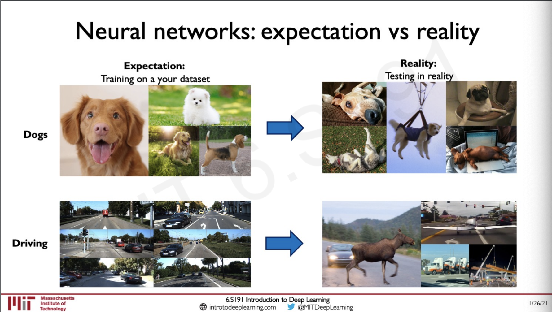
When we train our model we train them with very clean data sets as we can see in the left, like for the dog images but in the real world we would more likely to see something on the right or something that the model can never expect, this is completely possible not to be caught in a dataset but chances of them happening in real world are still high because we cannot predict what a model might encounter in the world. So we need to equip the model to tackle these situations and hence the necessity to understand the uncertinity.

All models are wrong, but some - that know when they can be trusted- are useful!

~ George E.P Box(Adapted)

The problem is that more than what we could expect knowing when we don't know is also really hard, even in real life there might have been cases for us humans when we are very sure that we might be doing something right with just our instincts but we could be actually be doing something very wrong.

Probabilistic learning

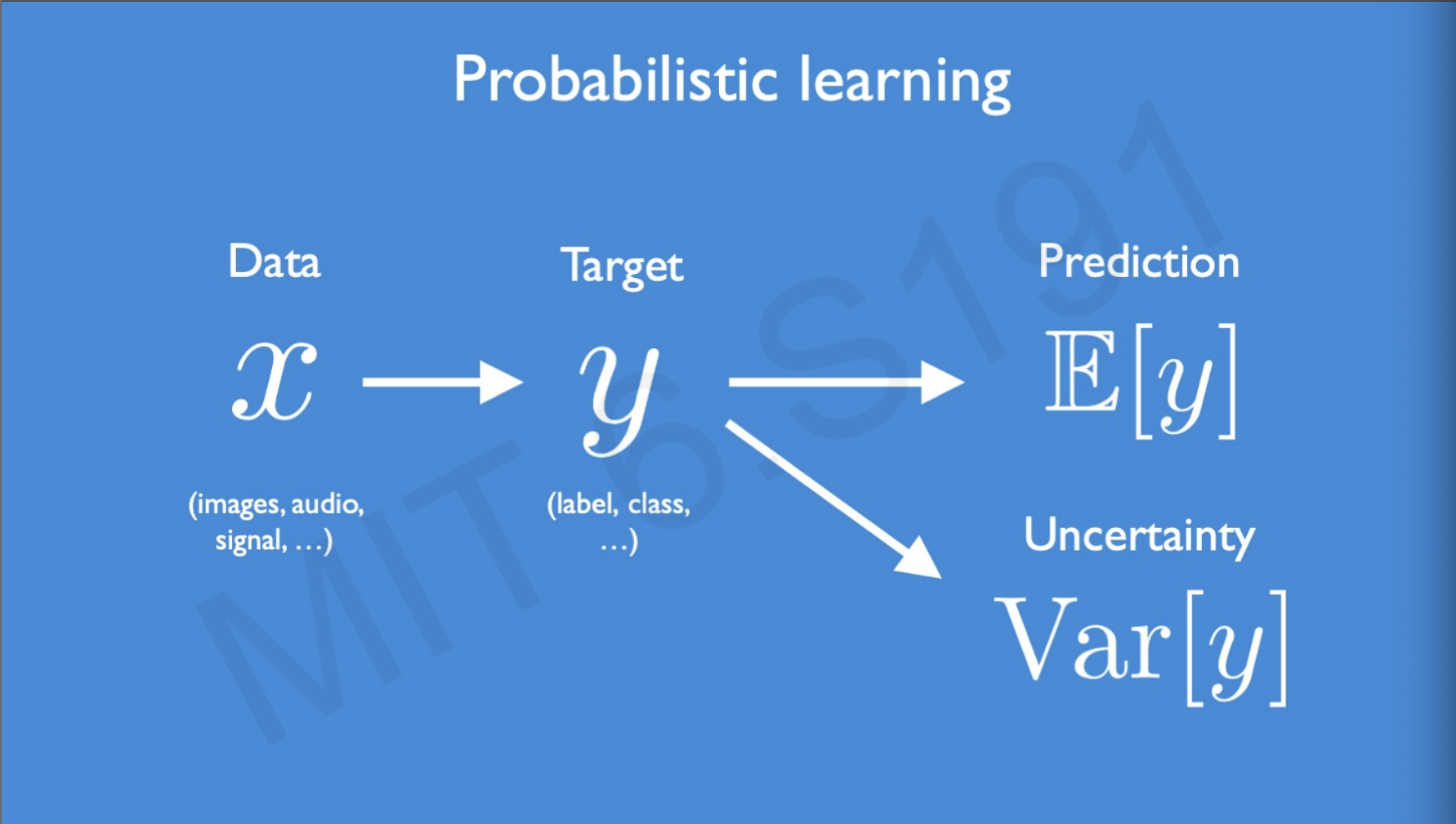
So far we have been training data in such a way that we have an input that is our data represented as <$x$ and our target $y$ and the idea is that we predict the expectation of y given the data x, apart from this our goal here is to also learn the uncertainty which is the variance of y.

This is similar to what we have seen before when we are given lets say an image of a cat and we need to predict if it is a cat or a dog with a neural network. The neural network does two kinds of prediction.

1. $p(y="cat"|x)$
2. $p(y="dog"|x)$

The probability distribution here is over discrete class categories.

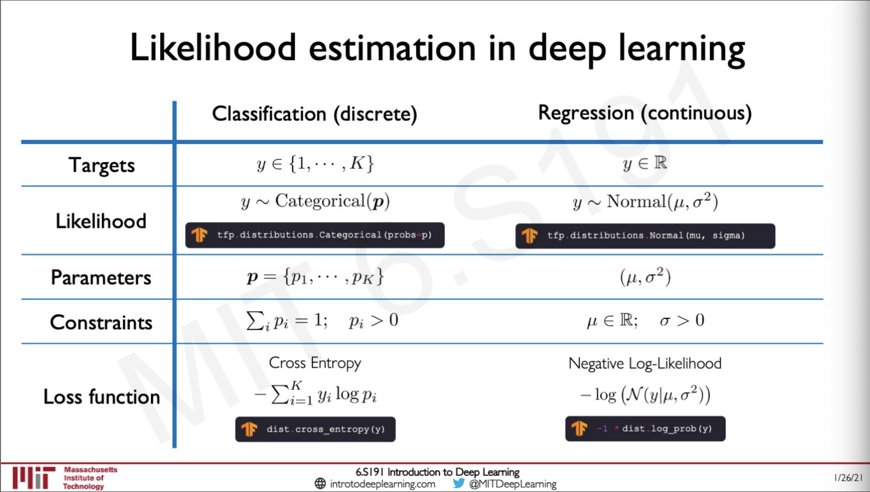
Discrete vs Continous class targets

Let's once again take closer look at how we did our classification for both discrete and continuous classes.

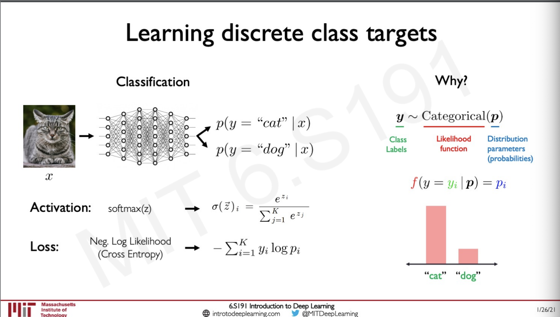
For discrete classes we are giving the output as a probability that is if it is a cat or a dog and as we know the probability is between 0 and 1 and we need to enforce these restriction for the same we have the softmax activation function and to follow the softmax and measure the likelihood for our data to be a label we have the loss function that is cross entropy.

For a continuous class,

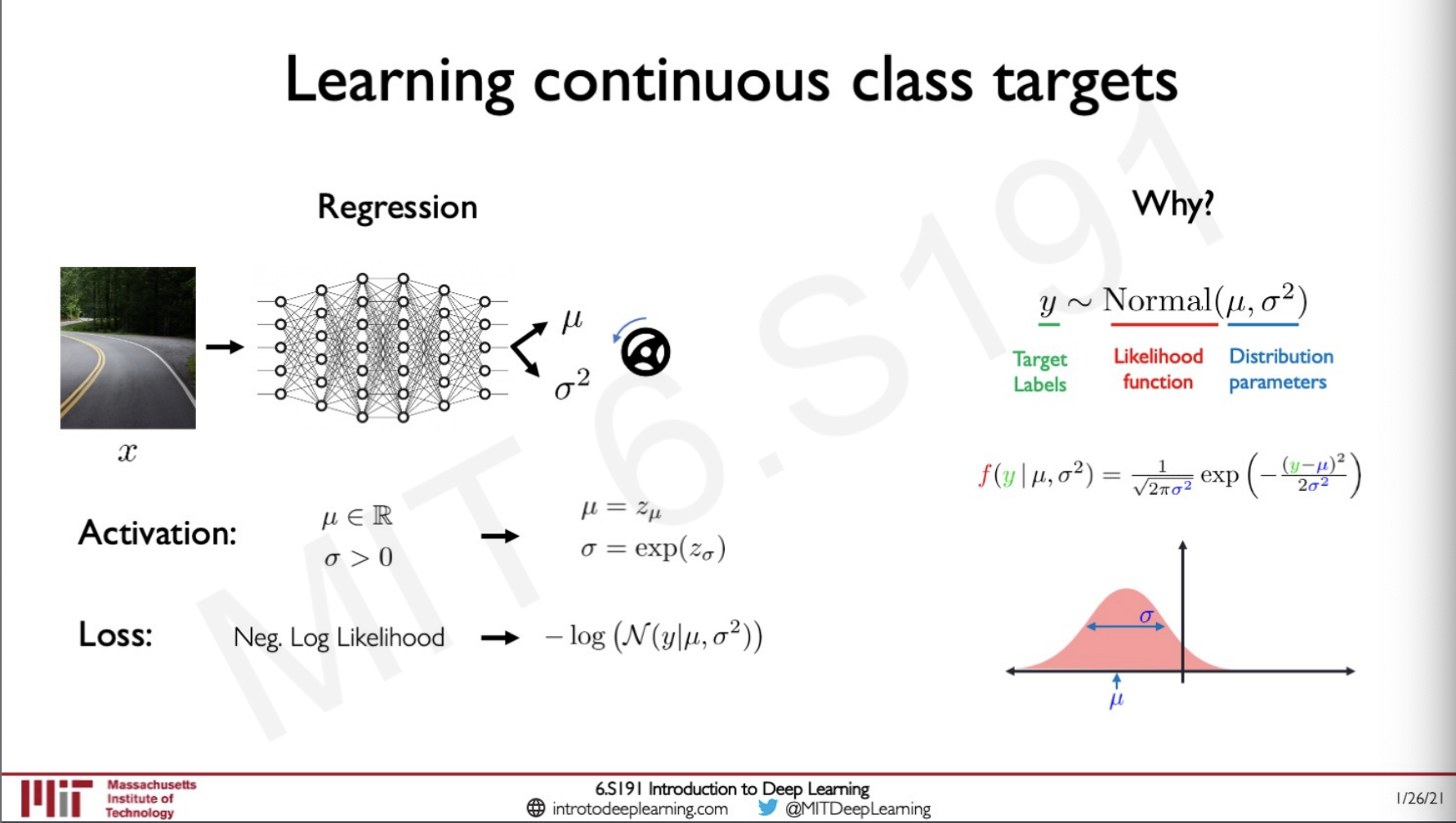
Here instead of classification, we would be doing regression and the thing about regression is that the output would be any number and this is an infinite set of possibilities which is not a good thing to be modelled by a neural network so we will have the output as a mean and variance so that we can sample from the probability distribution of these values assuming that the probability is Normal Gaussian. Here the activation is chosen smartly with some constraints that the variants should always be strictly positive and hence we use an exponential activation function. The mean does not have any restrictions. We also have a Negative Log-Likelihood loss we can use to see how good our model is training.

Likelihood vs Confidence

One of the key things that we should remember is that we should never mistake the likelihood or probability of a model for confidence.

What this means is that lets say we have a model that is trained to predict if an image is of a cat or a dog and the model actually performs really well.

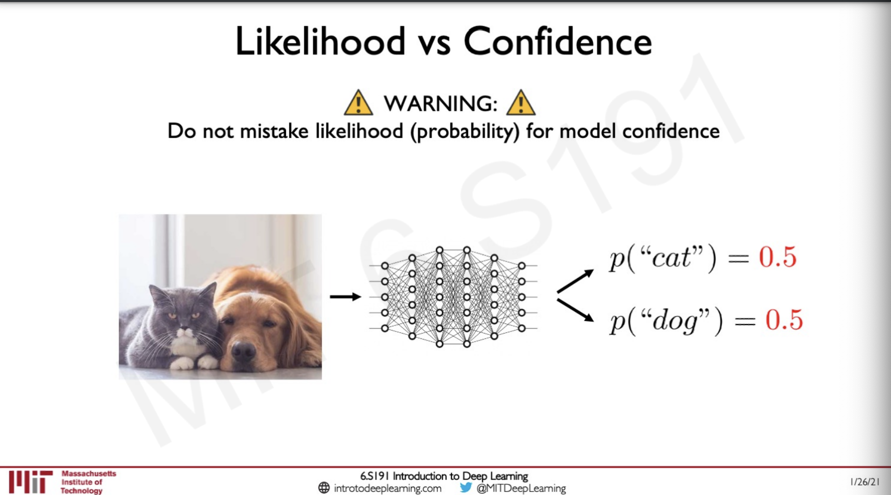
At this point we give the model with an image of a cat and a dog and the model recognises both features of cat and dog in the image and then predicts 50% chance for both, this does not mean that the model does not know if the image is not confident weather the image is of a dog or a cat but rather it knows it knows it found features of both.

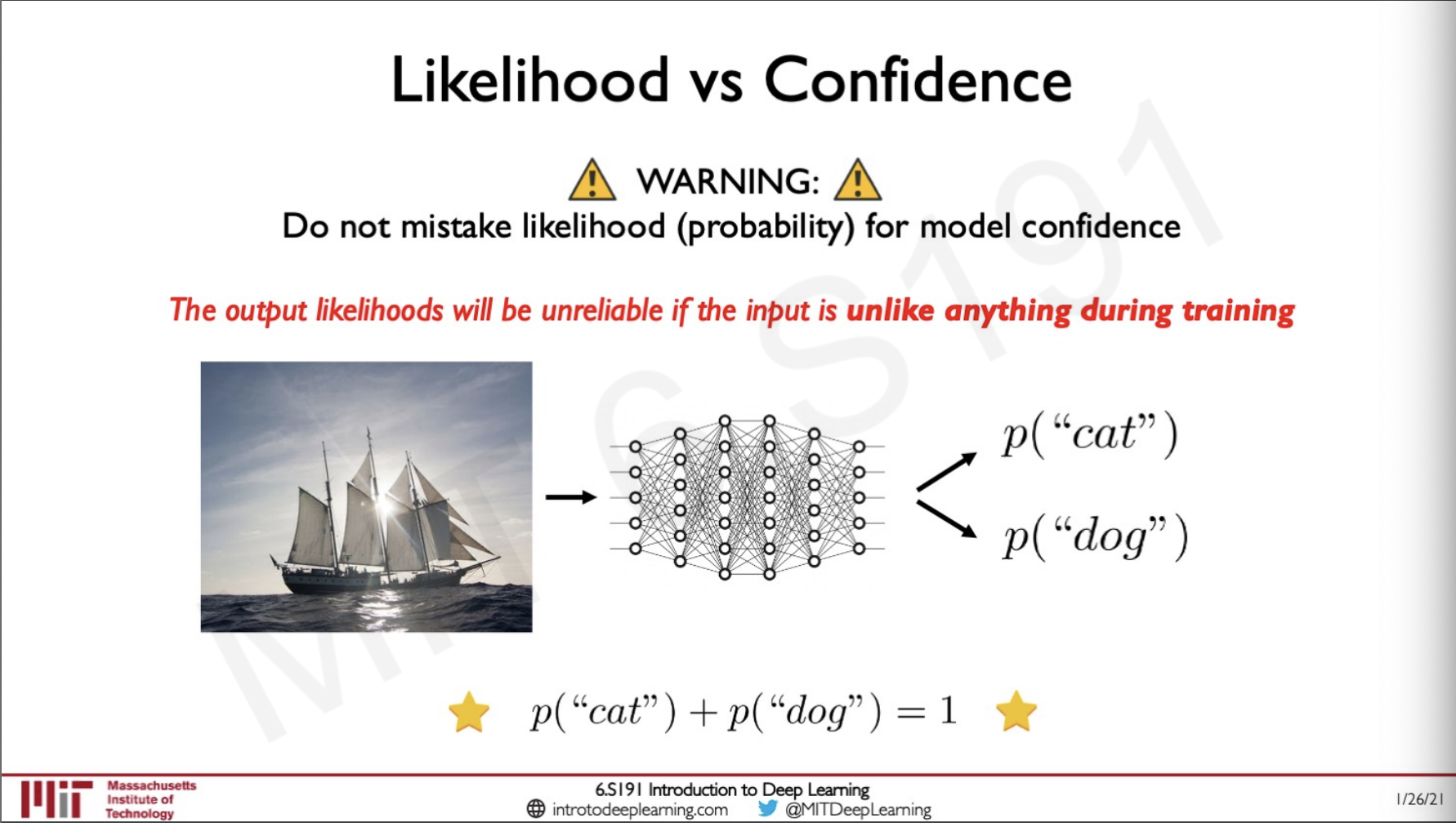
But now let us say we passed an image that is not at all related to something that the model knows but in this case the problem is that we have engineered the model in such a way that the sum of the probabilities should be 1 and here the model might go wrong and show that one of the either class with a greater confidence. This is not correct and we need to fix this somehow and that requires for us to understand uncertainties.

Types of uncertainty

We can classify unknowns into four categories,

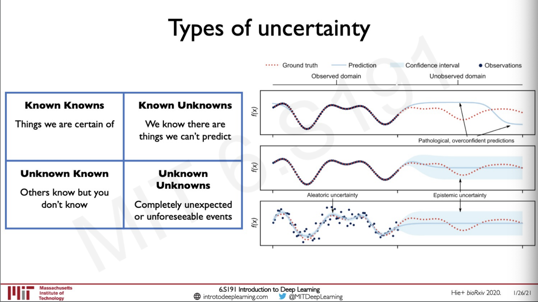
1. Known Knows - Let's say we are in an airport and we know that some planes are going to depart from the airport, these are known knows.
2. Known Unknowns - We cannot predict the time a certain aircraft is going to takeoff because of cases that the it might be delayed.
3. Unknown known - We do not know the fight schedule of another person.
4. Unknown Unknowns - There are things we have no clue about like if a meteor would hit the runway.

We can visualise these uncertainties as shown in the graph in the right side where the function is f(x) and we are trying to create a model to learn this function the successful part is under observed domain and the portion for where we do not have training data for is under unobserved domain. If we try to do prediction on the unobserved side the prediction would be very unconfident and these kinds of uncertainties are called Epistemic uncertainty where the uncertainty is in the model. If we have uncertainties in the model it is called Aleatoric uncertanity.

Aleatoric vs Epistemic Uncertanity

Aleatoric Uncertainty

• Describes the confidence in the input data
• High when input data is noisy
• Cannot be reduced by adding mode data

Epistemic Uncertainty

• Describes the confidence of the prediction
• High when missing training data
• Can be reduced by adding more data

While Aleatoric uncertainty can be learned directly using neural networks we cannot estimate epistemic uncertainty because it is more challenging.

One solution to this is to rather than training deterministic neural networks we can train a Bayesian neural network.

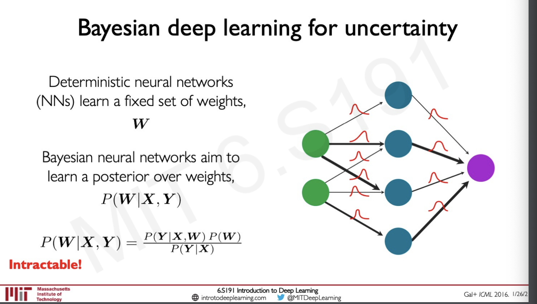
The idea here is that instead of the neural network learning some weights W it can learn posterior over the weights. A Bayesian neural network has a probability distribution attached to each of its layers and we perform multiple forward passes each time with a new sample of weights and biases so that we can learn if the uncertainty will be high at which particular distribution. The problem with this is that this mostly works only on toy examples and it is intractable.

One fix to this is to approximate through sampling.

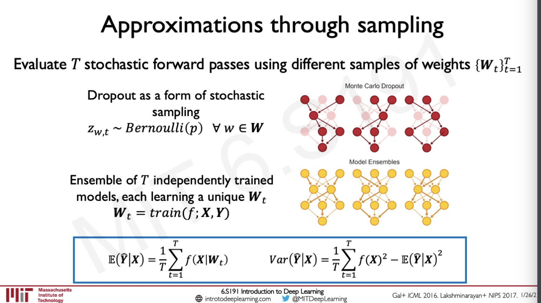
Here we are using dropouts as a form of stochastic sampling turning off nodes and then sampling the data.

Another method is to do ensemble of T independently trained models where each of the model is learning a unique set of weights.

In both the cases we are estimating both the Expectation as well as the Varince.

Some of the limitations of Bayesian deep learning is that,

1. Slow - Requires running the network T times for every input
2. Memory - Stores T copies of the network in parallel
3. Efficiency - Sampling hinders real-time ability on edge devices
4. Calibration - Sensitive to choice of prior and is often over-confident

Beyond sampling for approximating uncertanity

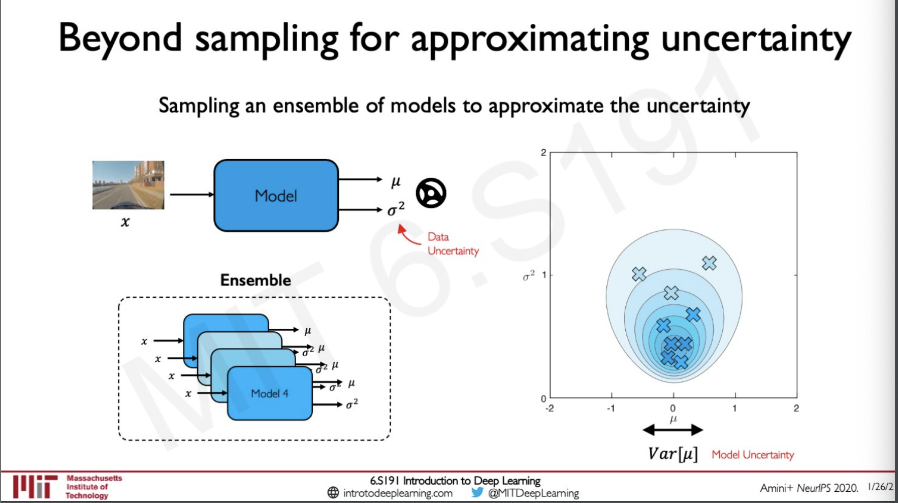
Let us look back into the example of a driverless car here the model takes in an image as input and then the $\mu$ here is the angle at which the steering should turn and the $\sigma^2$ is the epistemic uncertainty. When we train this model in an ensemble we get an estimate of where the mean and variance of each of the value is going to be and we can plot this on a graph as shown, if the points are closer together it means that our model is performing well and if not otherwise.

What this means is that even though we are training many models we are getting similar probability distribution of the points are closer together.

The uncertainty that we are sampling is actually drawn from some unknown distribution so instead of sampling what if we can learn these distributions directly.

Evidential deep learning

The idea here is to treat the learning process as evidence acquisition.

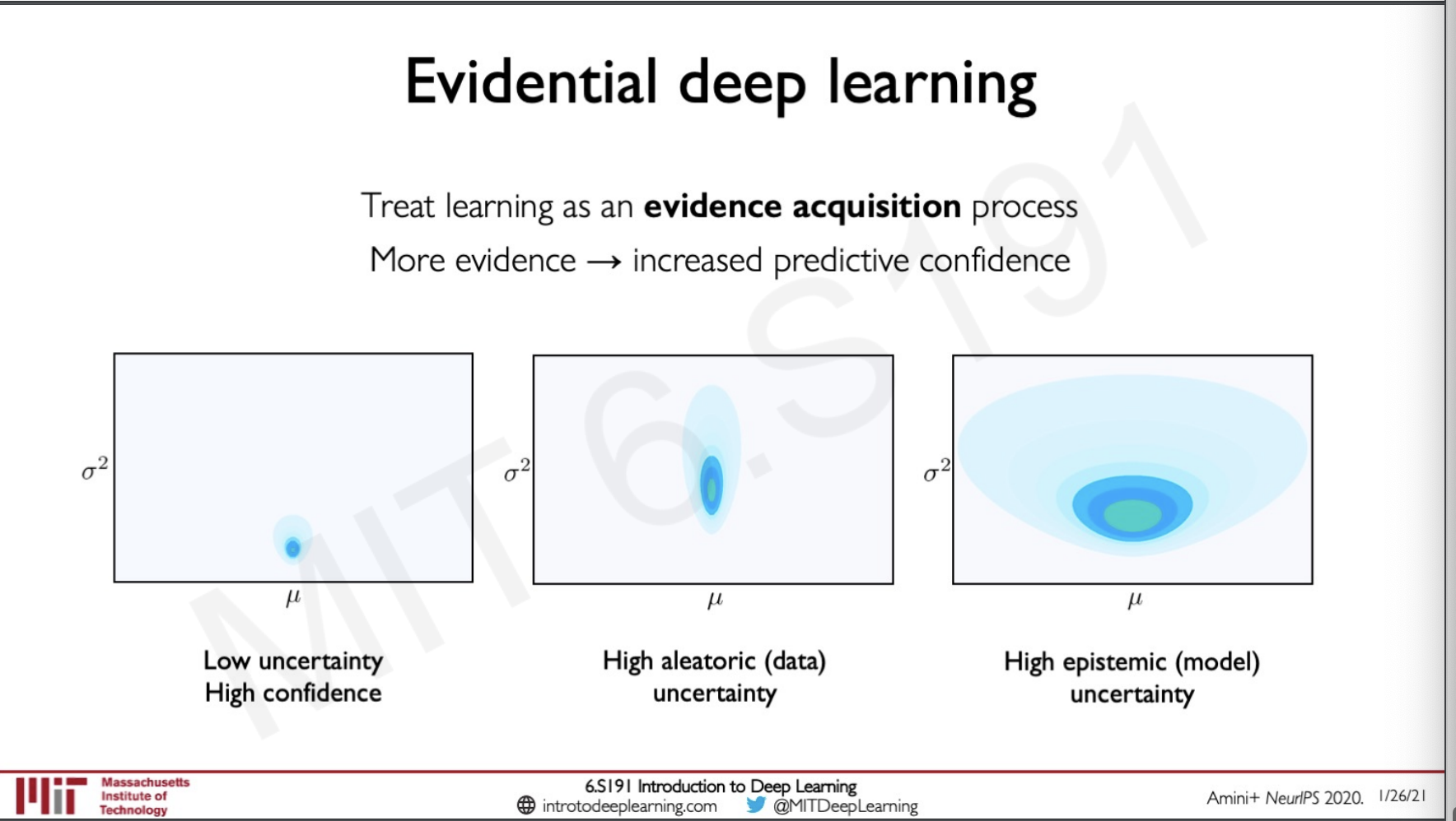
As we can see with the determination of the $\mu$ and $\sigma^2$ we can plot this and interpret what kinds of uncertainty are we dealing with both aleatoric and epistemic.

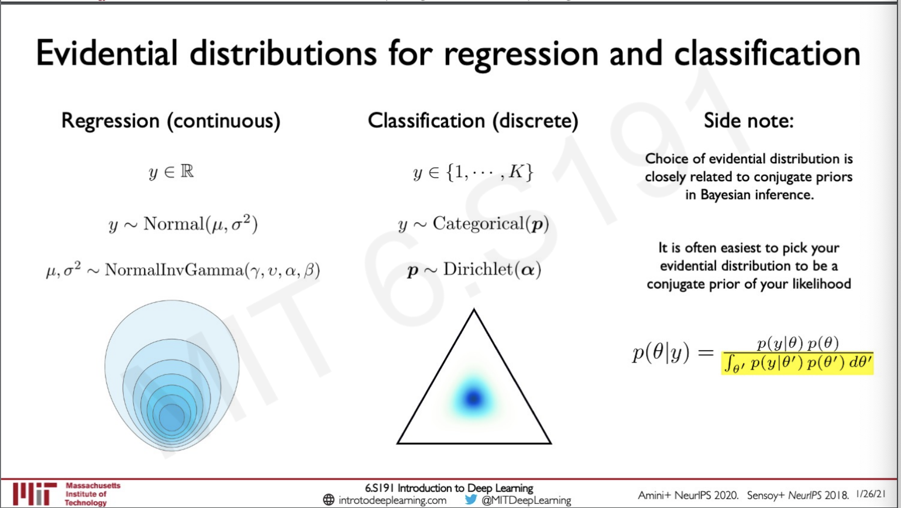
Evidential learning for regression

To clearly understand evidential learning we need to keep in mind one thing that is the $\mu$ and $\sigma^2$ we are generating here are distributions that are representing some other distributions that we have over our data.

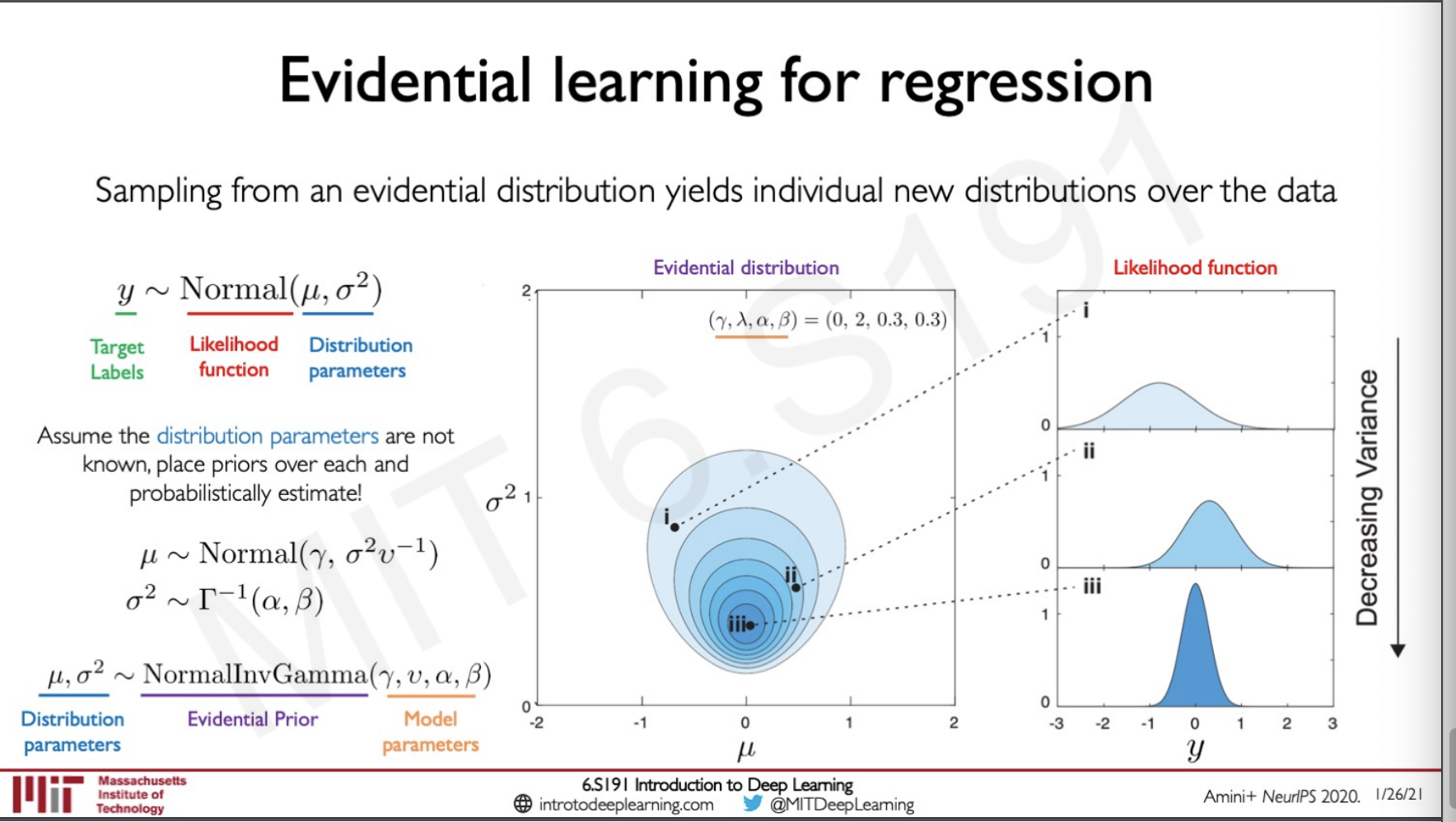
So how we can utilise this is by taking out the old technique and then placing a prior over the values for estimation. By placing these priors we are able to get values for our distribution parameters and as we can see from the picture on the right sampling from each of these data points actually gets us an underlying probability likelihood function.

Evidential learning for classification

For the classification side of things also our theory remains the same we are sampling a distribution of another distribution.

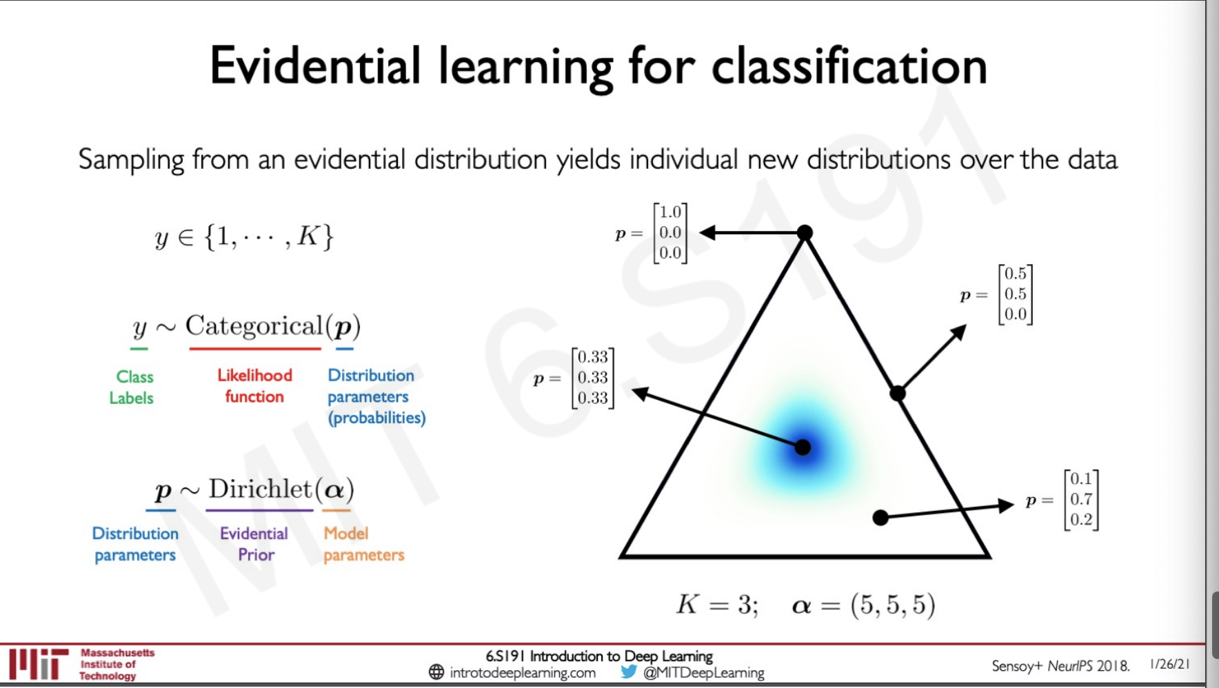
Here our evidential prior would be Dirichlet and we would be sampling from a model parameter $\alpha$ which is k in number each representing a class. Let us say that we have 3 possible classes which can be represented by a triangle simplex and the blue mass is representing our probability mass. Sampling from this triangle will give us the categorical probability distribution.

• Sampling from the middle of this simplex would represent equal probability for each classes.
• Being on one of the corners will show one of the mass being on one class and 0 for the other two.
• Sampling from anywhere else would show the sampled probability distribution for each of the classes each summed to 1.

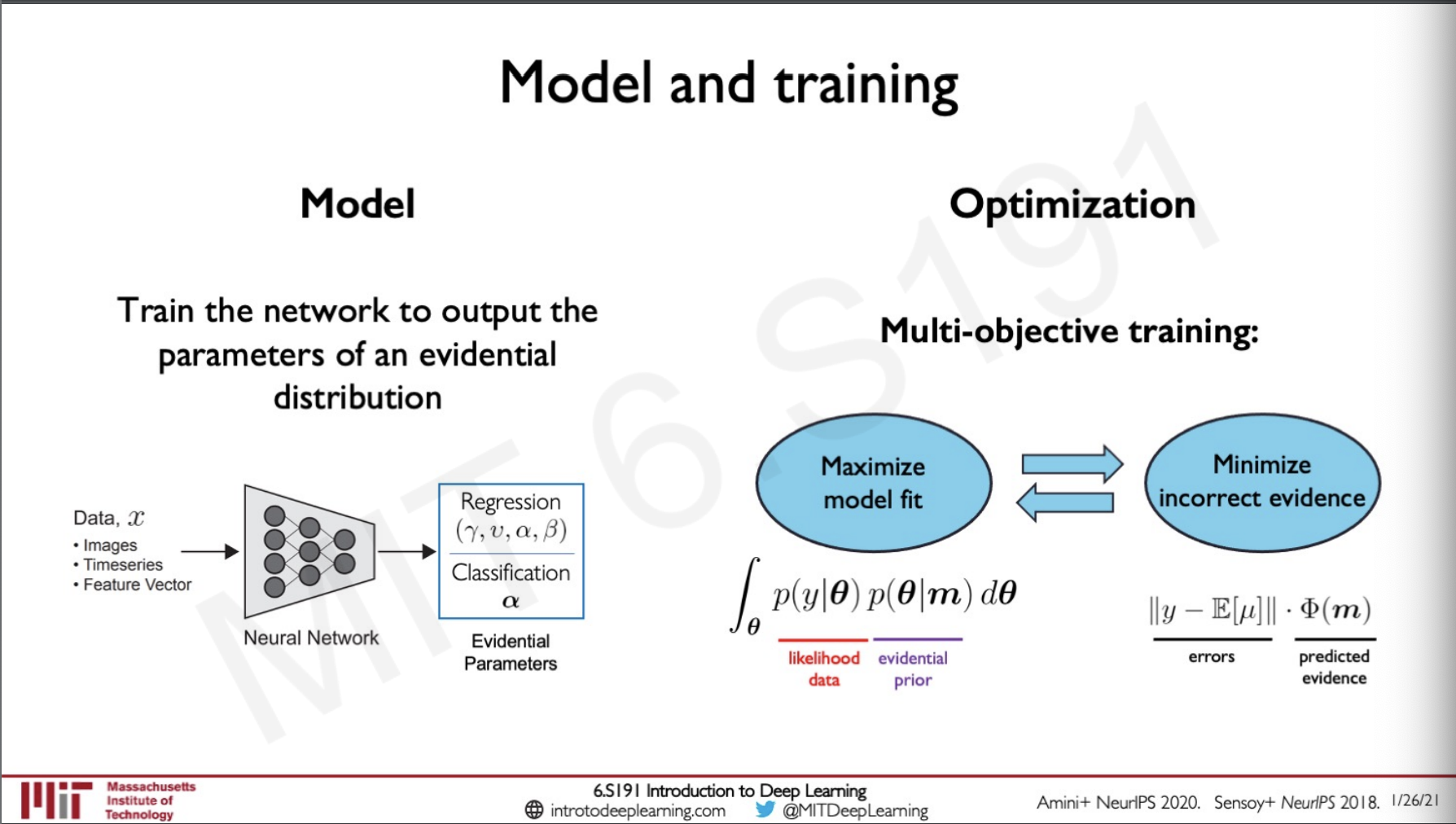
Model and training

The models are trained to output the higher order parameters,

These models were tested on Toy examples and the following was the result.

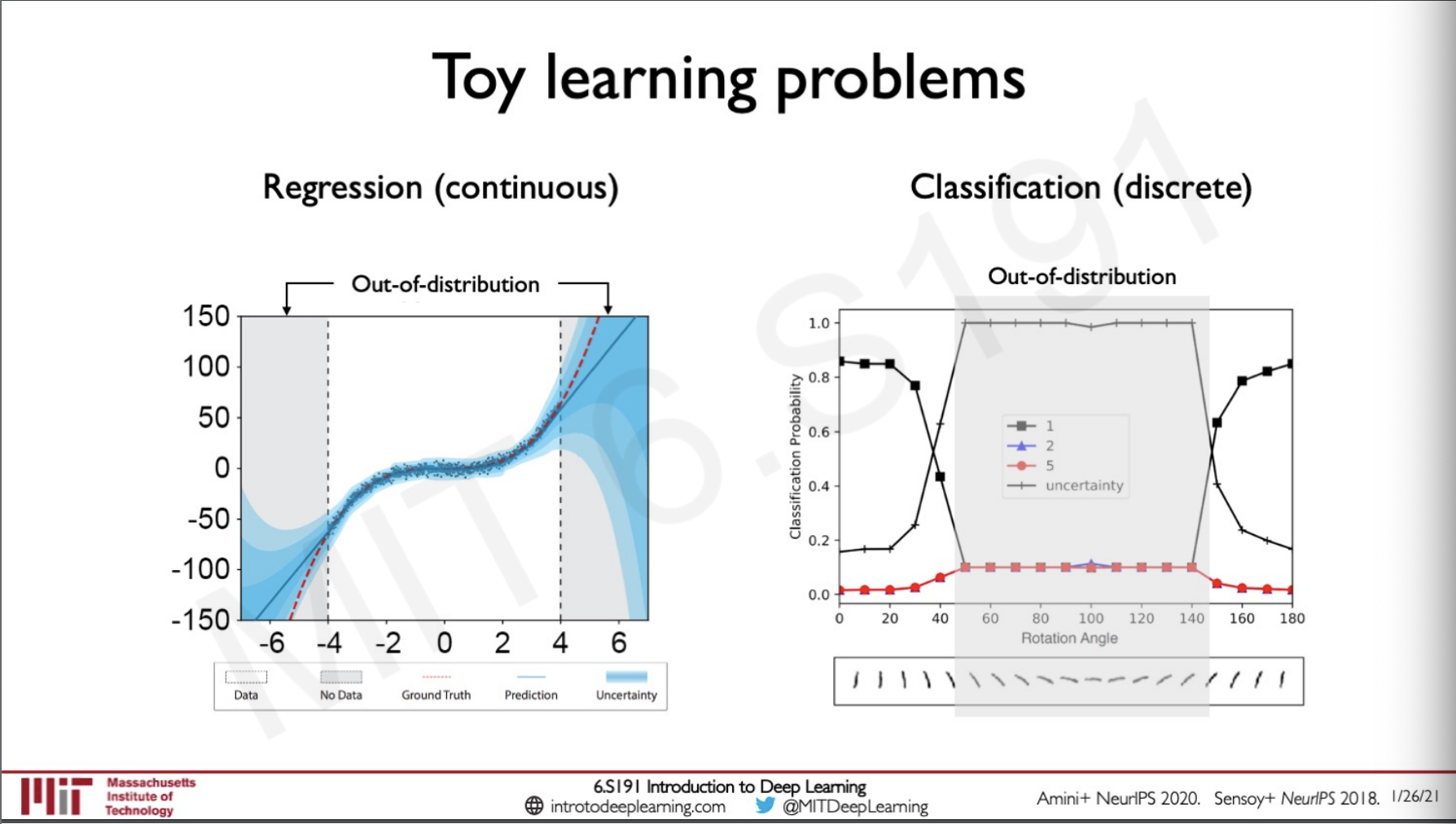
For regression when the data was given out of distribution region the model showed a greater uncertainty which is what we need and the same goes for classification where the MNIST dataset digits where rotated and was passed into the model which also showed a higher uncertanity.

Applications of evidential learning

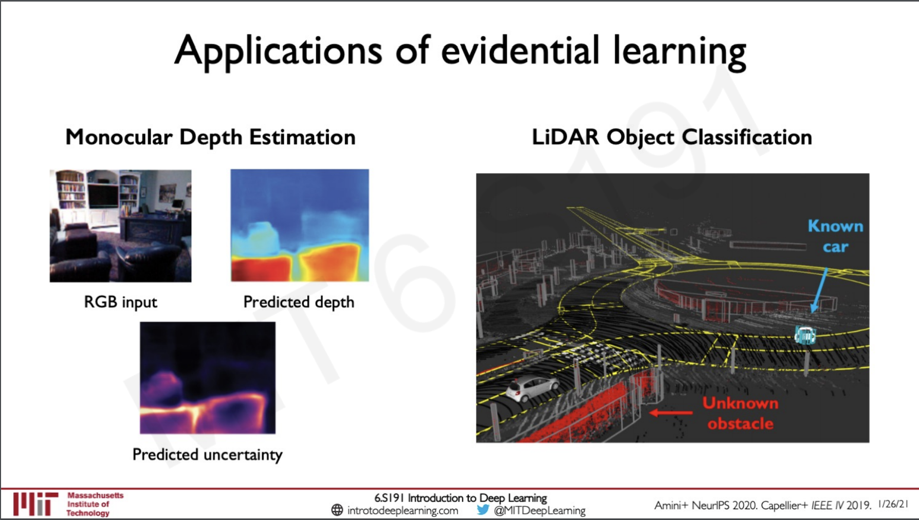
The Monocular Depth Estimation is the task of estimating scene depth using a single image. This is a regression problem because the value of the pixels can have infinite values.

Evidential learning has also been used in Classification for objects from a point cloud.

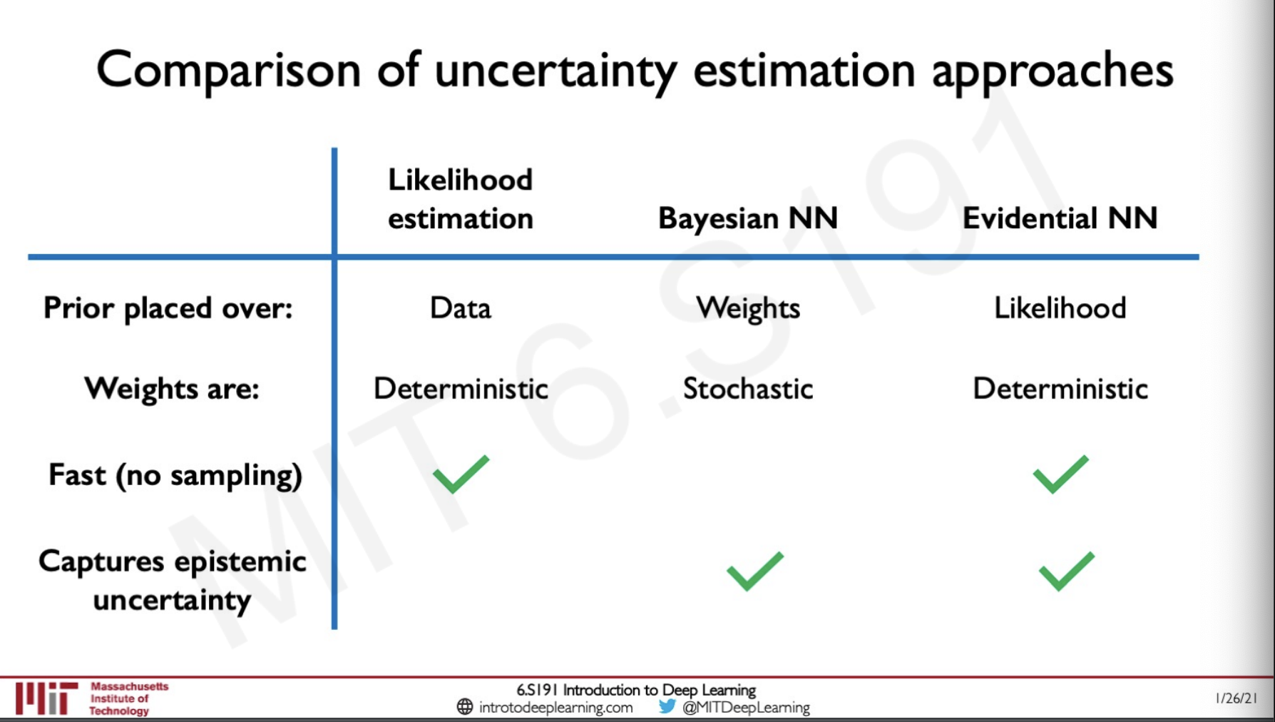
Comparison of uncertanity estimation approaches

Sources

MIT introtodeeplearning : http://introtodeeplearning.com/

Slides on intro to deep learning by MIT :http://introtodeeplearning.com/slides/6S191_MIT_DeepLearning_L7.pdf