Part 4 : Following along MIT intro to deep learning

Deep Generative Modeling

Introduction

Until now we have explored various methods in deep learning which we can use to do a task such as classification and regression where we have some data and do some prediction over that data. The scope of deep learning does not stop here it is beyond this as well we can generate synthetic data and like faces or images.

Supervised vs unsupervised learning

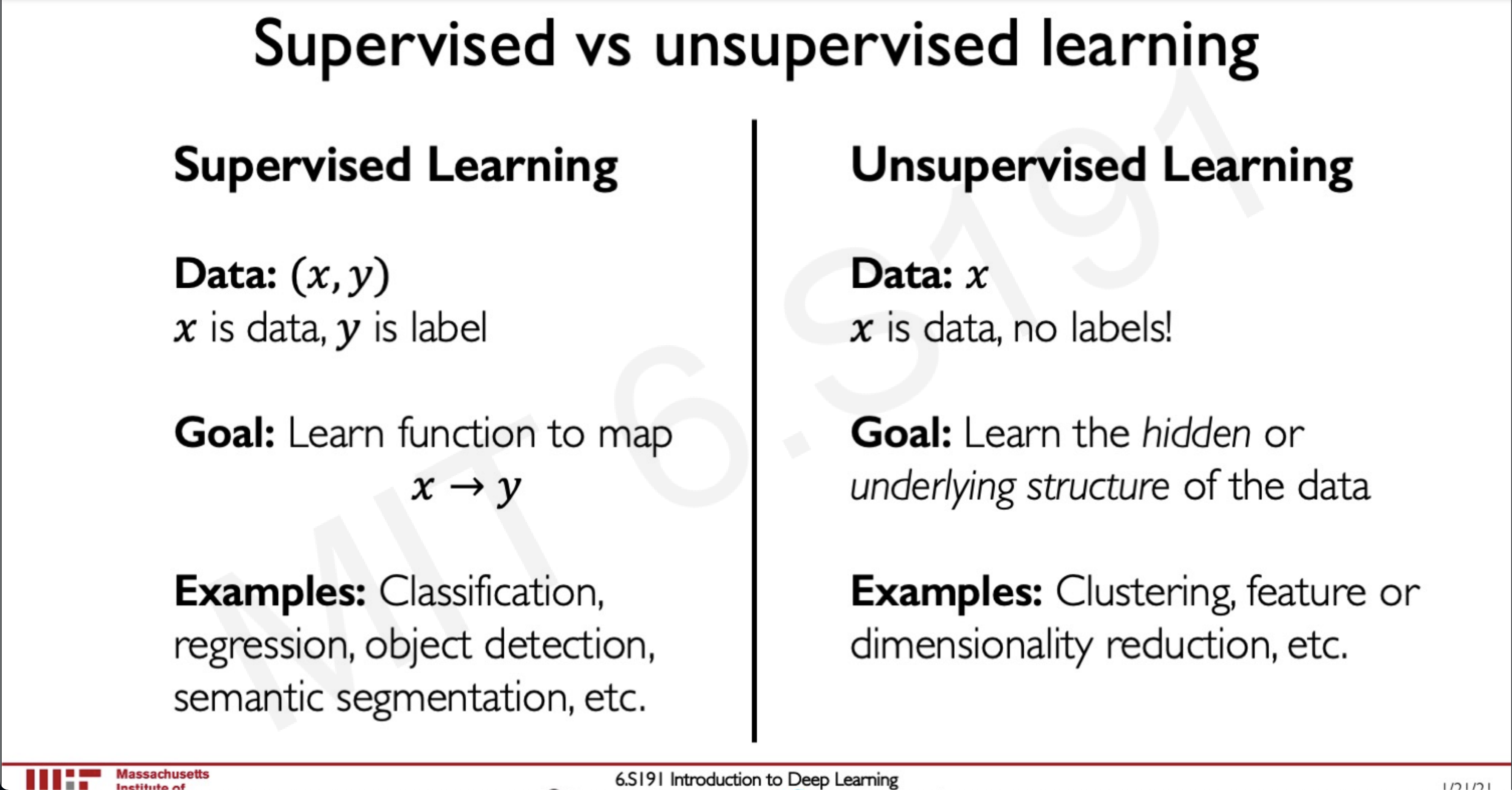
So far we have seen supervised learning where we have data and a label and our job is to create a function that maps these data to these labels.

Now we will take a look at a different approach we have some data and we need to find some patterns inside this data without being given any labels this is unsupervised learning and generating synthetic data falls under this category.

Generative modeling

The goal of generative modelling is to take as input some distribution and learn a model that represents that distribution.

We can do this in two ways,

Density Estimation

We are given a sample of data and we have to learn the probability distribution in that sample of data.

Sample Generation

Here we are not only given a input sample and we learn the probability distribution form this sample but we also use these samples to create a new data

The training data $\sim P_\bgroup data \egroup (x)$
The Generated $\sim P_\bgroup model \egroup(x)$
The challenge is how can we learn $\sim P_\bgroup model \egroup(x)$ when we are given $\sim P_\bgroup data \egroup (x)$

Why generative models? Debiasing

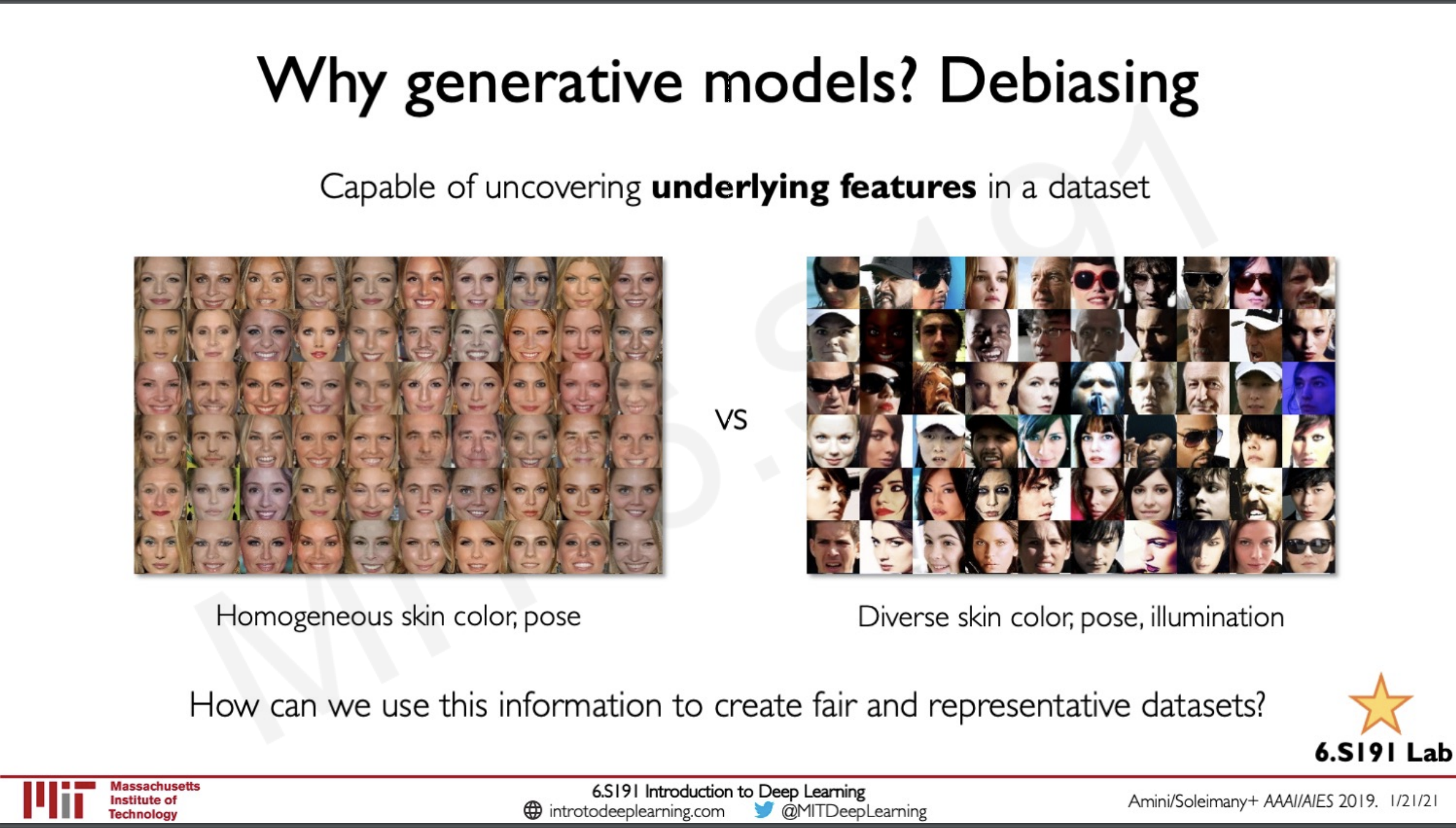
One of the problem that generative models can solve is to de-bias a dataset, most of the dataset that is available these days from which we are able to train another model from are generally biased what this means is that they may be having homogenous skin colour; homogenous pose etc.. This is a very big issue as in real life the data is not biased so we need some form of mechanism to solve this bias one would be to train a GAN that is able to de-bias these dataset to ensure that they are fair and representative to the real world.

Another use of generative models would be during outlier detection, during the training phase of a model that is used in self-driving cars. Here there may be outliers like let's say a plane flying across in the sky which is captured by the camera or harsh weather or even pedestrians these outliners can be detected with the help of a generative model from the distribution and using these outliners we can train the model to improve even more.

Latent variable models

We would be seeing mostly two latent variable models

1. Auto-encoders and variational Auto-encoders (VAEs)
2. Generative Adversarial Networks (GANs)

What is a latent varibale

By definition, latent variable means variables that not directly observed but are rather inferred from other variables that are observed. This can be described by a very good story from the Myth of the Cave.

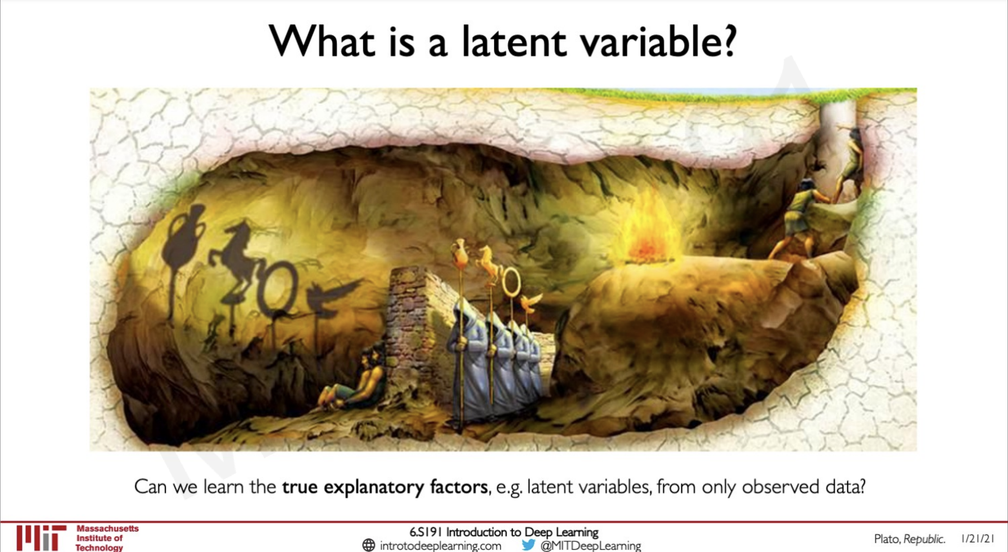
Here there are some prisoners who are facing the opposite side of the wall and they are observing shadows casted by objects that are behind the wall. The prisoners can understand what the objects are by looking what they can infer from the shadow but they are not able to know the actual features as they are not looking at the objects directly. The objects are latent variables and the shadow is another variable that is observed from which they can infer information about the latent varibales.

Our task is to train neural networks that can observer latent variables given an observed data. (Think of this from the perspective of what un-supervised learning means)

Autoencoders

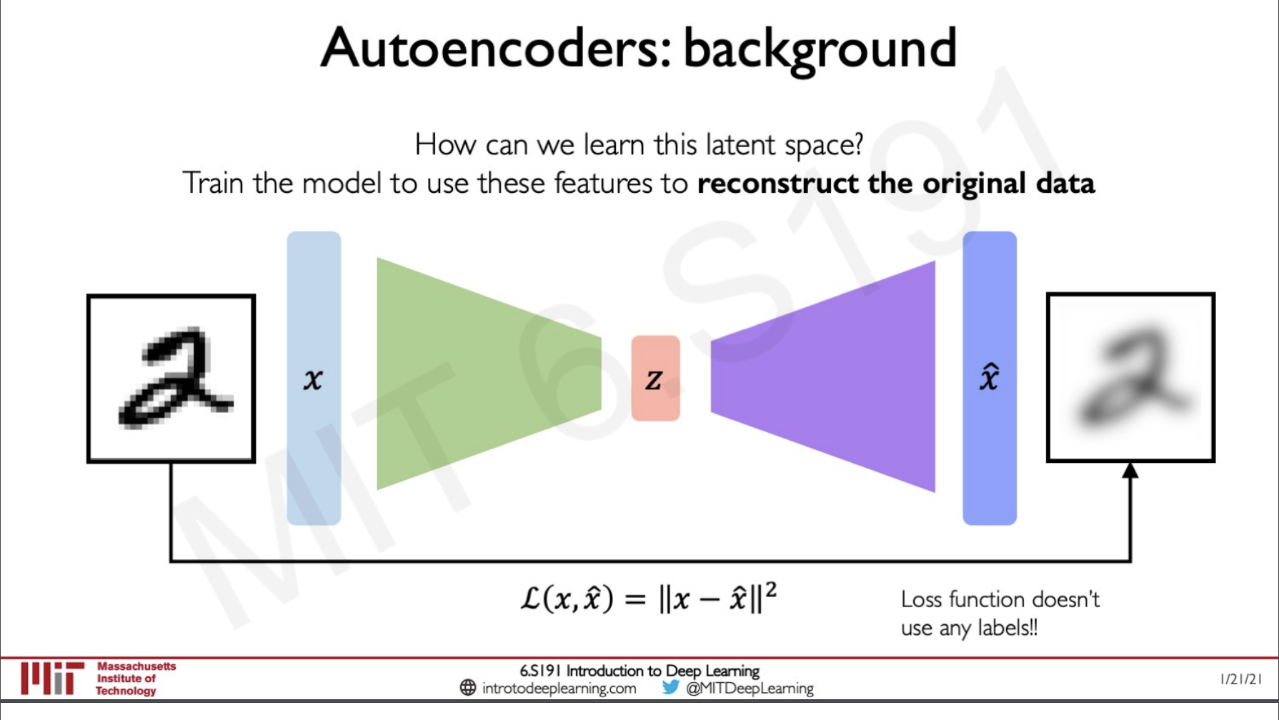
In order to learn the underlying pattern in the data, we can pass the data down a neural network like a CNN which is doing dimensionality reduction.

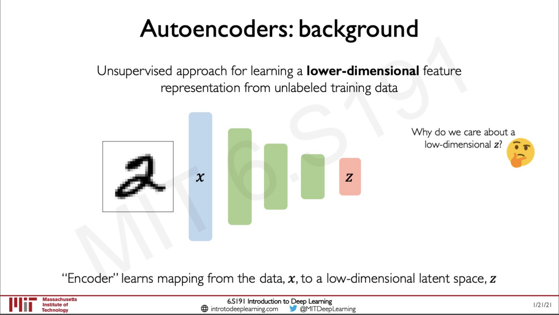
Here we can see that we are giving the input image 2 into the layer x and then it is being passed down through a convolutional neural network (of the encoder) and then finally it is given as output in the layer z where we can get the feature-rich compressed representation of this data.

Since we are doing an unsupervised approach where there is no concept of any labels so how can we know if the network is giving the right output at z, simple we do the opposite of the encoder network we create a decoder that takes in the latent vector and the increase its dimensionality to reconstruct out the image.

We determine the loss by measuring the distance between the image that is given to the network $x$ and the output of the image that is $\hat\bgroup x \egroup$ since the image is the reconstruction of the original image. Here the latent variable $z$ is a compressed representation of the image.

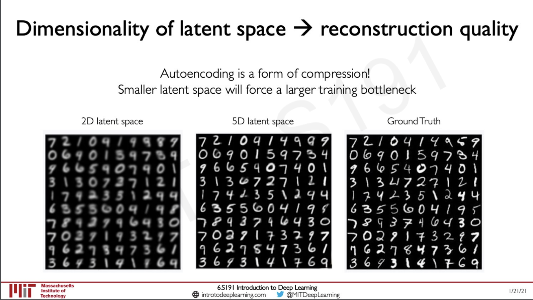
If we add very fewer layers to out network in the encoder or decoder side we will lose the reconstruction quality of the image because the more hidden layers we have the more minute patterns can be observed by the model and this would create a representative latent vector from which we can reconstruct the image.

Variational Auto-encoders (VAE's)

When we take a close look at the normal autoencoder we saw before we realise that this is a deterministic model as long as we pass in the same input we get the output as a reconstruction of the image

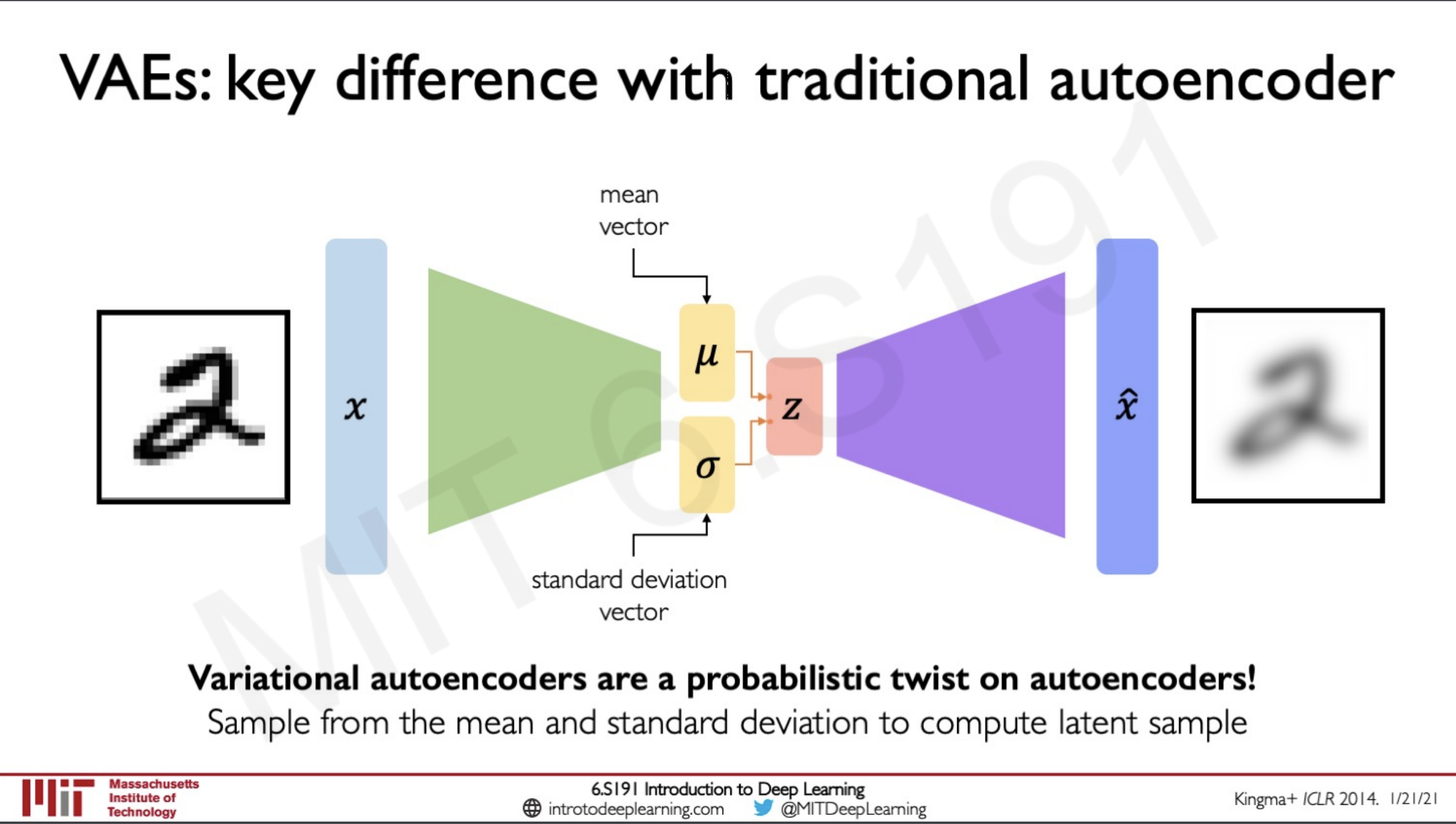
Variational autoencoders are a probabilistic twist on auto-encoders they introduce a twist to the network by creating a sample from the mean and standard deviation to the computer the latent samples. They introduce stochasticity to the sampling process that is instead of learning what the latent variable is they have two more vectors that learn the mean and standard deviation such that instead of learning what the vector directly is it learns the probability distribution that is underlying in the network and try to produce another probability distribution that is similar to the learned distribution.

VAE optimization

The optimisation process in VAE is done in two steps

1. The encoder computes $q_\bgroup \phi \egroup(z|x)$ where the input given to the network is x and it is trying to predict the probability distribution z for the weights given by $\phi$
2. The decoder computers $p_\bgroup \theta \egroup(x|z)$ where the input given to the network is z and it is trying to predict the probability distribution x for the weights given by $\theta$

The loss is computed by summing together two factors.

The reconstruction loss is similar to what we have seen in autoencoders it is the log-likelihood loss between $||x- \hat\bgroup x \egroup||^2$
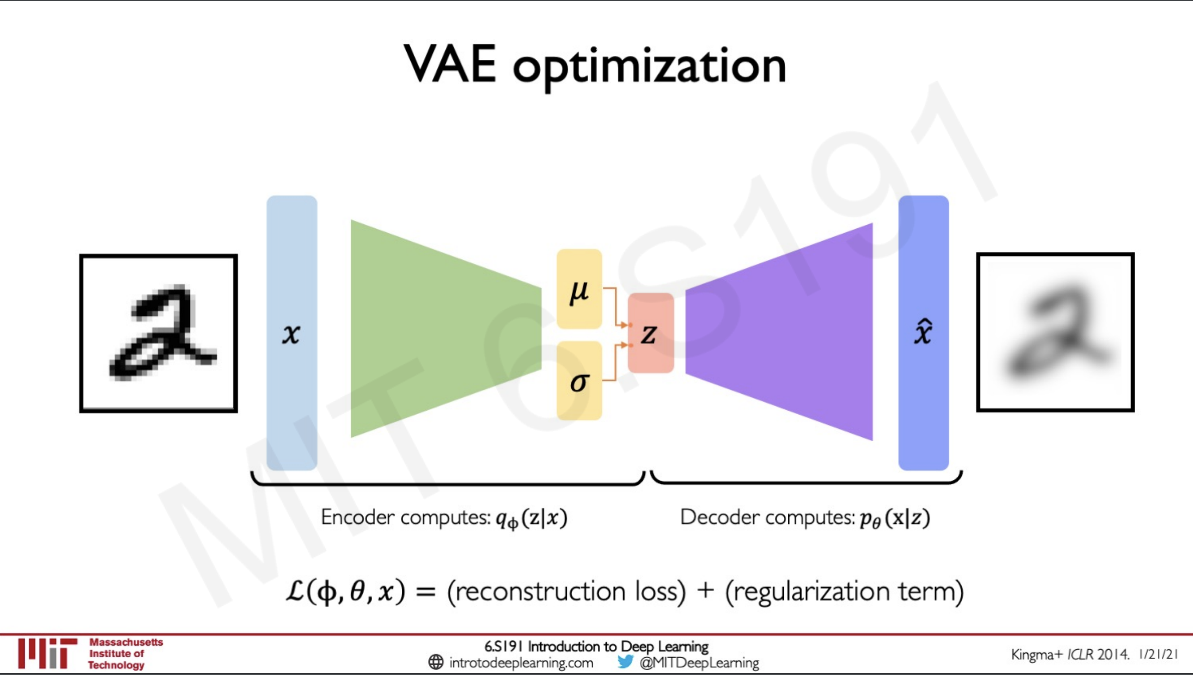
The probability distribution $q_\bgroup \phi \egroup(z|x)$ is a newly computed distribution z given the data x. What this enforces is that we are placing a prior on the latent space z this is to make sure that the distribution would be made to look like what we want it to be like.

The model will enforce the distribution it learns to follow the prior we are applying to it, this prior is denoted by $p(z)$

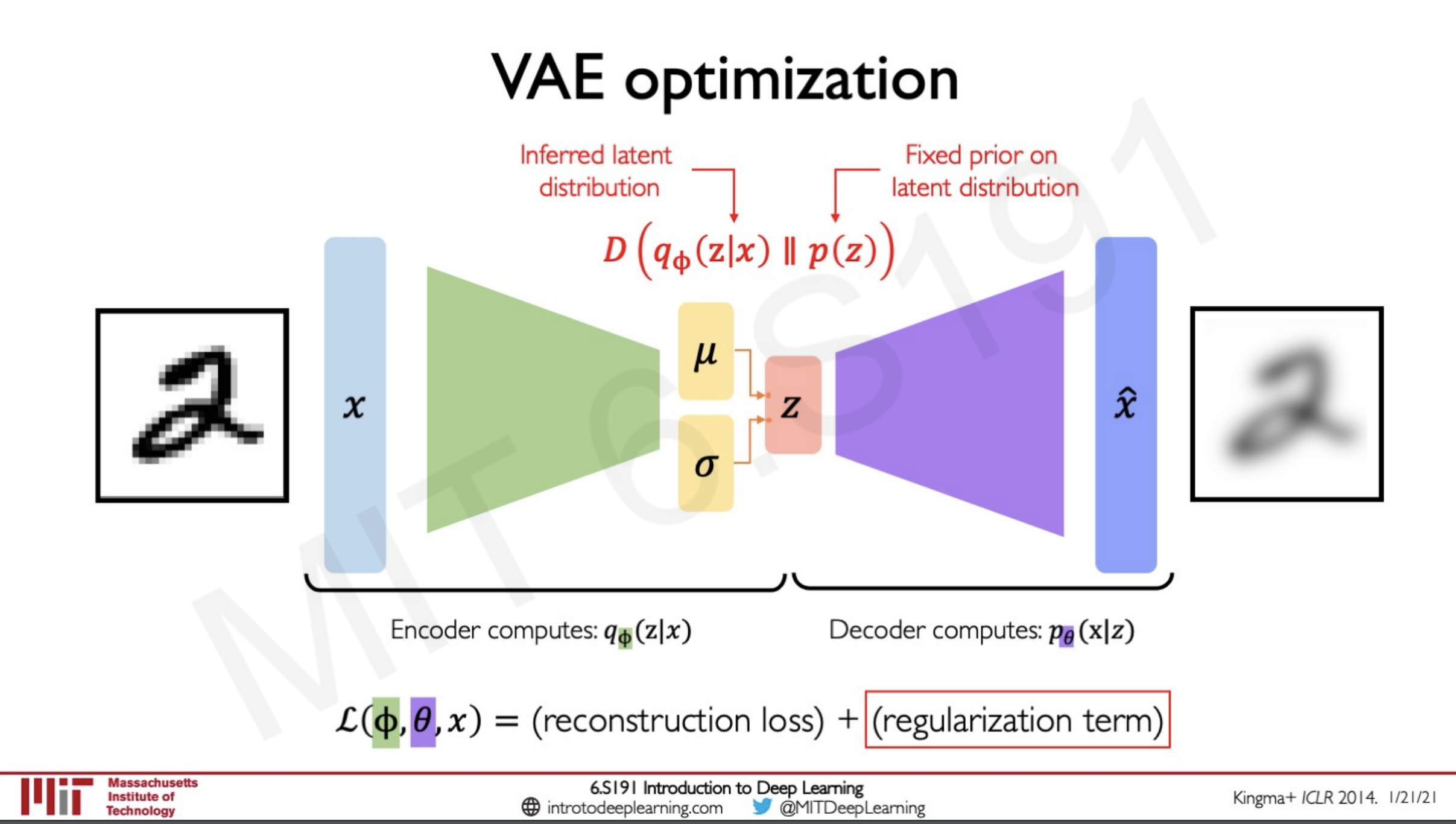
What the function D does here is a minimisation of the probability distribution we are learning and the prior that we are placing on the network. This would prevent the model from overfitting to the distribution of the latent space and would adapt to once that is similar to the prior.

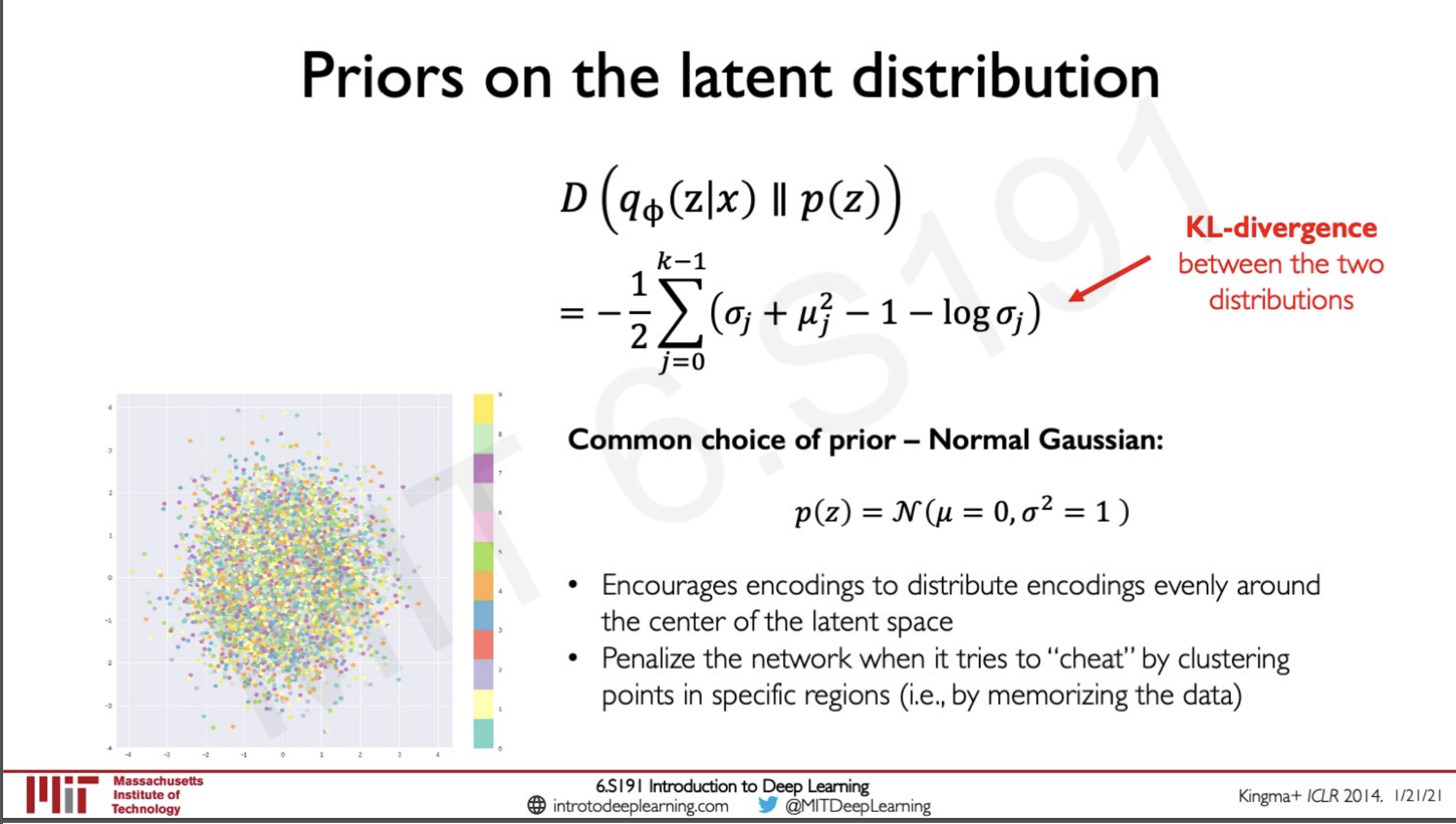
Generally the prior used as a regularisation for our network is a normal distribution this ensures that the network encourages the distribution to be around the center of the latent space. This also ensures that the network is penalised if it tries to cluster the points in specific regions by memorising the data and intern overfitting the model.

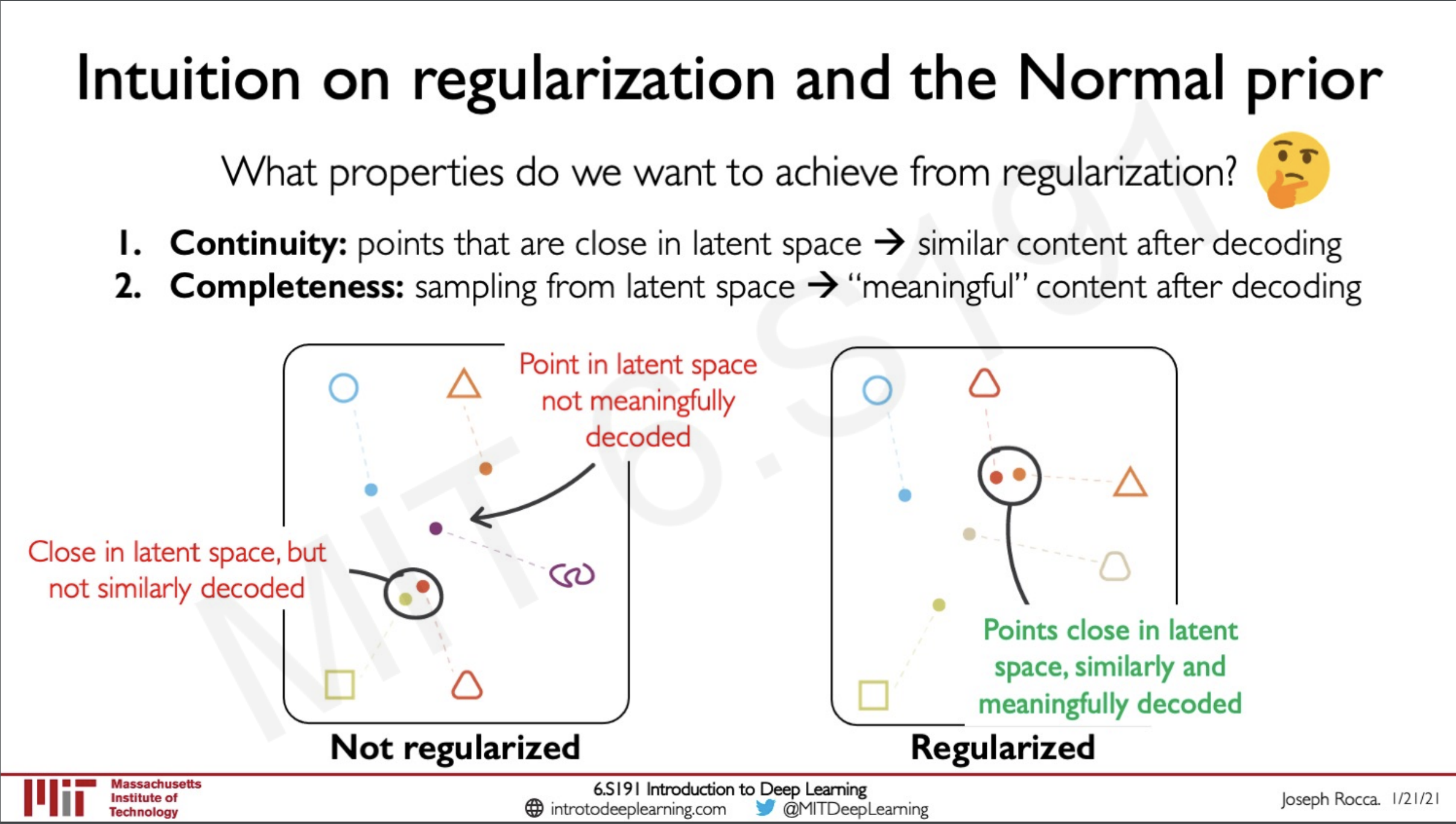
So now the question is why do we need to do this regularisation in addition to finding the probability distribution, remember we are not computing the probability distribution directly we are learning it and what this means is that there might be chances that it might learn the wrong way and this is why we implement the regularisation specifically in our case right now the normal distribution.

If the distributions not regularised the points that are close in the latent space may not be having similar decoding we ideally want similar things to be groups together and that is the case here as well we need the points to be grouped in such a way that adjacent things are representing similar objects when decoded. This is where regularisation comes to play if we are using the prior to be a normal distribution this would make the results follow the latent space to follow the same pattern as well.

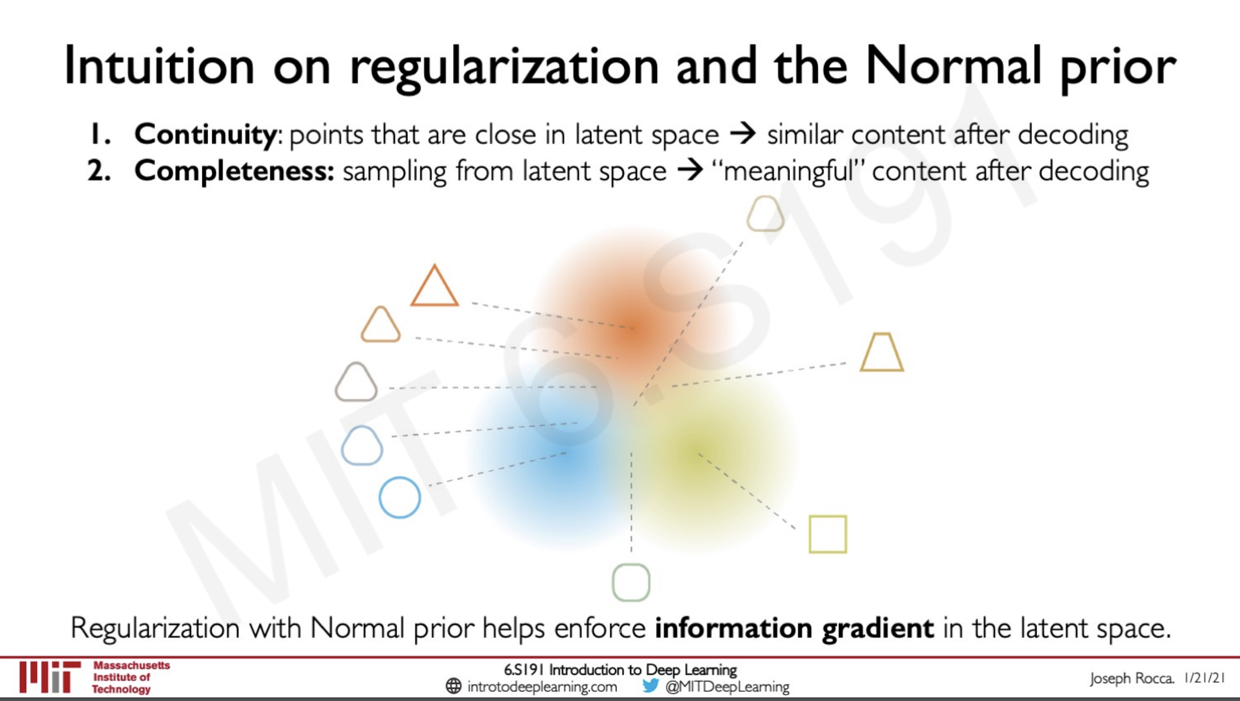
As we know in a neural network the data is propagated as gradients and using a regularisation on the gradients help it to cluster similar information together.

The problem with this approach is that we cannot backpropagate through a sampling layer and we need deterministic layers to undergo backpropagation.

Reparametrizing the sampling layer

So now what we have to do in order to do back-propogation is to reparametrize the sampling layer to be deterministic this can be done by

• a fixed $\mu$ vector
  
• a fixed $\sigma$ vector but this vector is scaled by a random constant $\epsilon$ drawn from a prior distribution (gaussian normal)

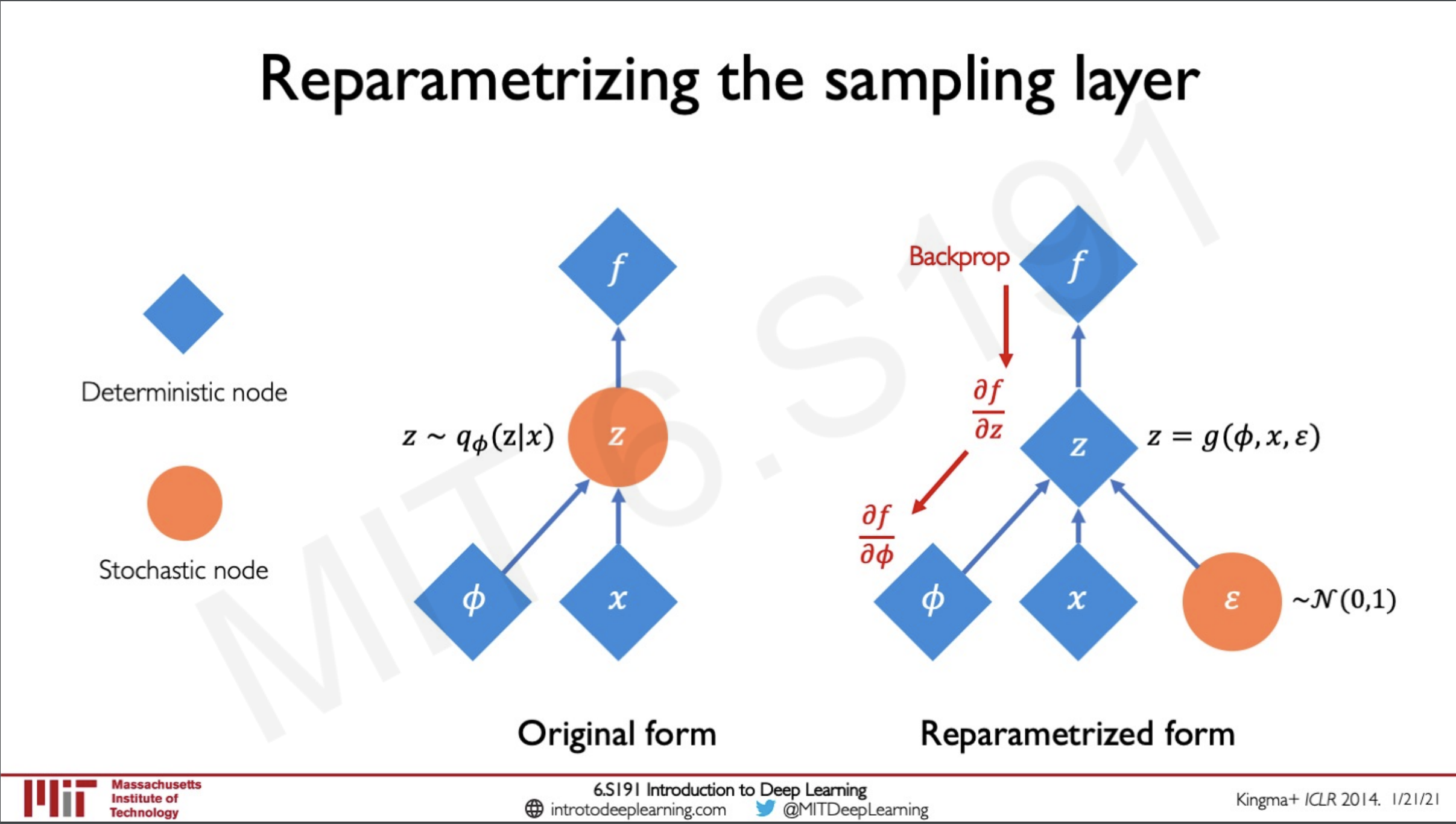
We can see here a comparison between the normal form and the new reparametrized form in which we can make the z node deterministic and we have modified the function to sample from the weights $\phi$ the input $x$ and the distribution function $\epsilon$. Here we are able to do the backpropagation down the nodes easily since they are deterministic layers.

Latent perturbation

The good thing about this is that we can fine tune a particular variable in our latent vector to and pass it through the decoder to generate different outputs this means we can understand particular changes like change in head-pose.

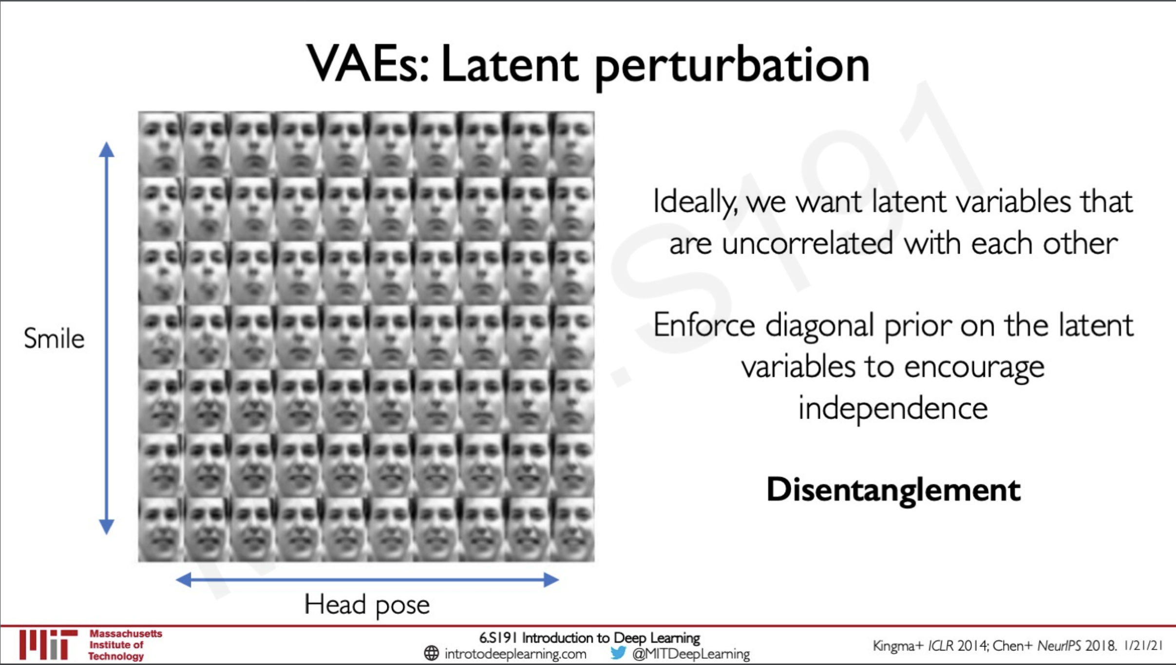
But the issue is that ideally we need these variables to be untangled that is each variable should represent only one feature if we change that variable it should reflect change on that feature here we can see a plot of Head pose v/s Smile this should not happen ideally.

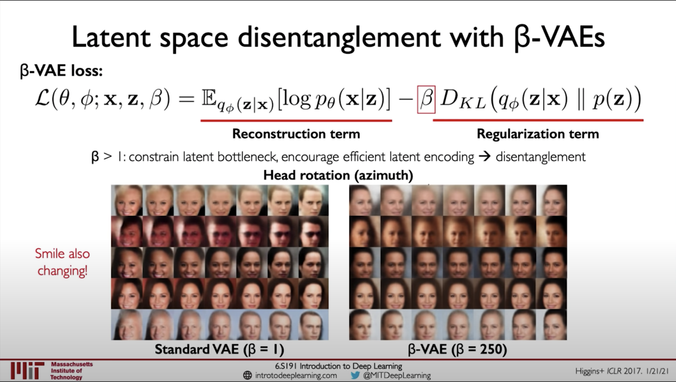
A technique that is known to work is that in have a value beta that controls the regularisation term. This acts like a bottleneck to the regularisation term and hence disentanglement of the latent variables.

Why latent variable models ? Debiasing

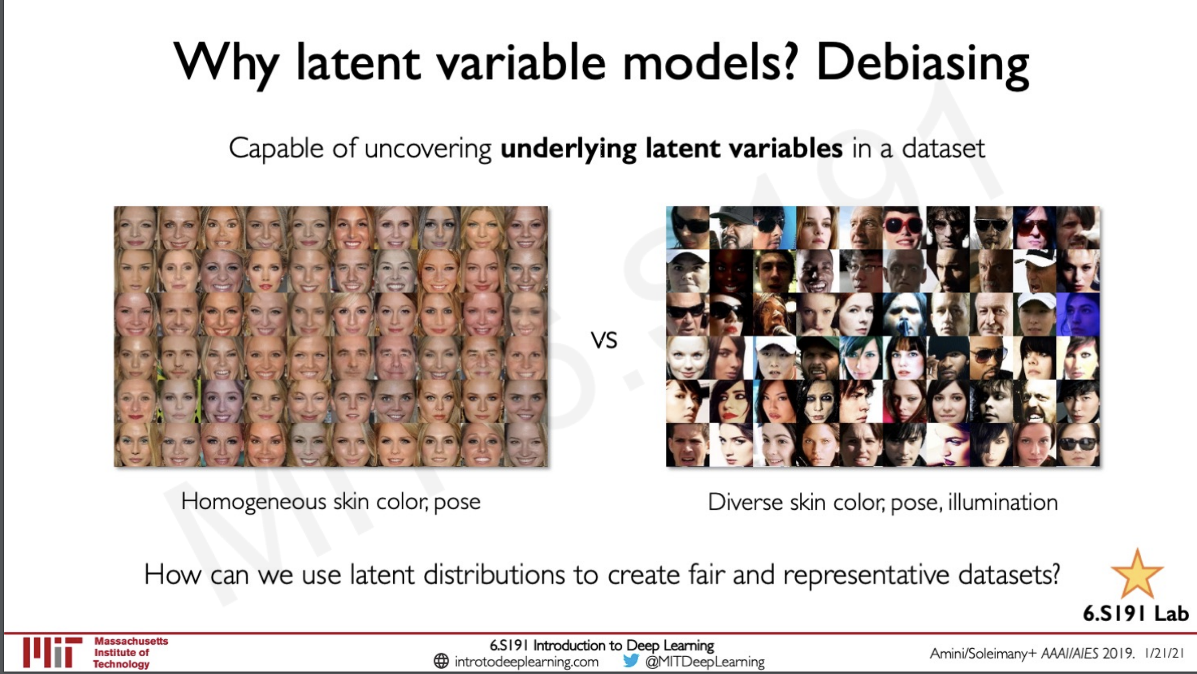
The datasets that are currently used mostly have some features that are either overrepresented or underrepresented like homogenous skin colour, pose etc... VAE's can actually be trained in such a way that it learns automatically which of these features are Biased and automatically de-bias them the cool thing about this is that we don't need to specify which of these latent variables are biasing but the network would automatically learn these biased features and de-bias them. The use of this is that we are able to create datasets that are representative of the real-world data and this intern would help us train models that can be deployed in the real world.

Generative Adversarial Network (GANs)

What if we don't need the model density but just generate new samples only, the idea here is to sample from nothing that is noise and learn a transformation to the data distribution.

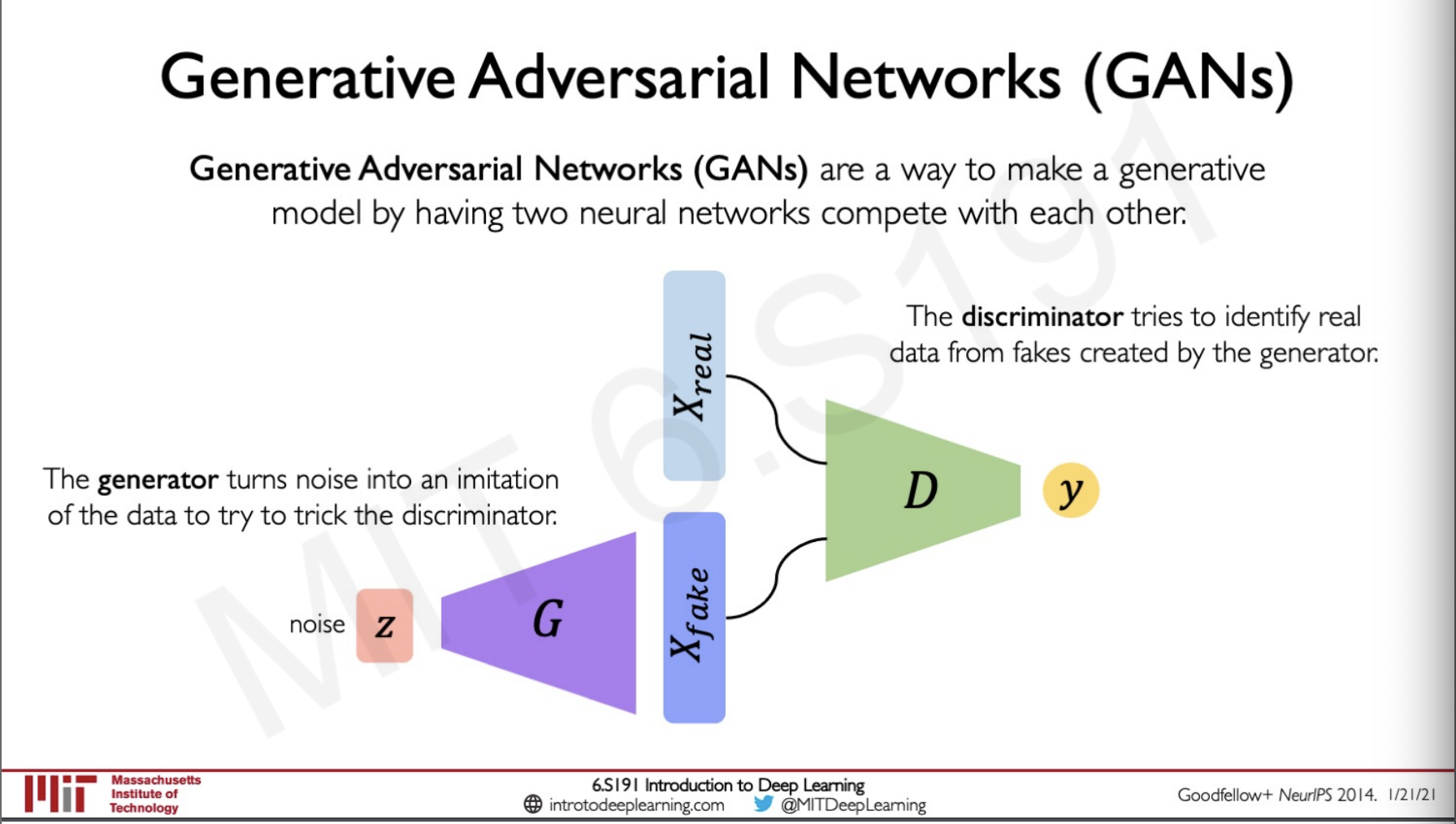
GAN is an efficient way to train such a network the idea is to have two neural networks to complete against each other the first network takes in a noise and try to generate a fake image the second network takes in the fake image and the real image and try to identify if the fake image is real or fake the generator tries to fool the discriminator and the discriminator try to outsmart the generator and thereby both the network learn to improve each other.

Training GANs

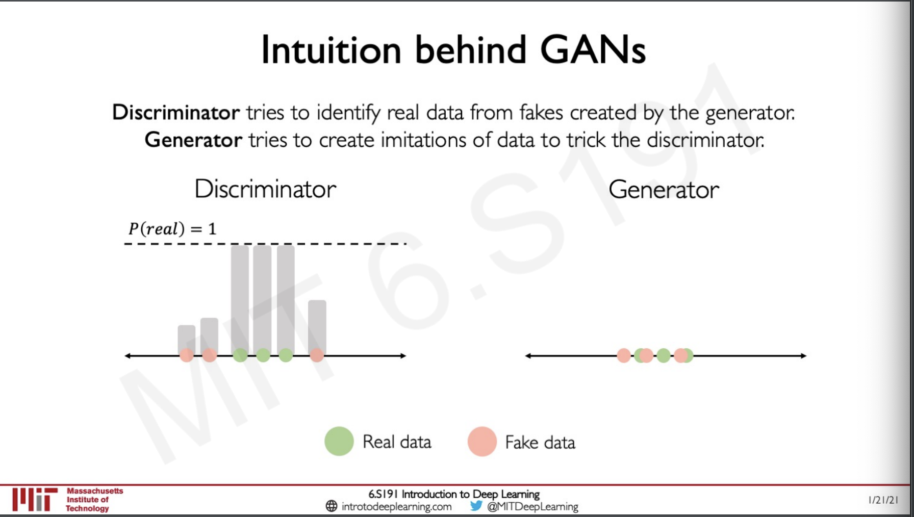
As we have said earlier the goal of the generator is to generate fake data that looks real and food the discriminator and the job of the discriminator is to discriminate of a data is real of fake.

So what is the global optimum for the data distribution we have created.

Lets first look at the loss for the Discriminator

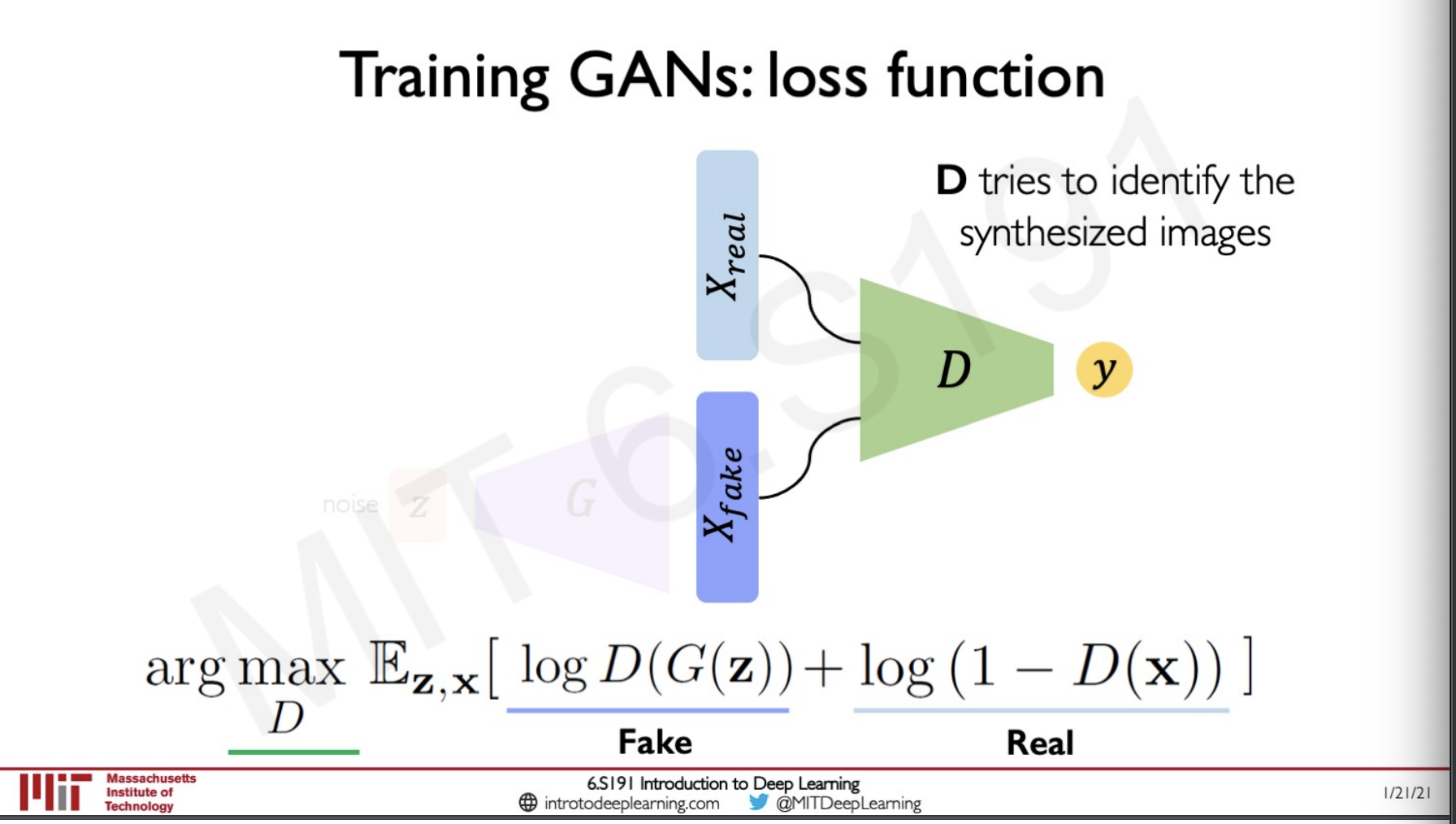
This is similar to the corss entropy loss,

We have to maximise the probability that the fake data is identified as fake

The $D(G(z))$ is the discriminators estimate the take fake data is actually fake

$D(x)$ is the discriminators estimate that a real data is fake subtracting it with 1 will give if real data is real.

We are doing a arg max to estimate the maximum estimate of real is real and fake is fake.

On the generator side this should have the adversarial effect,

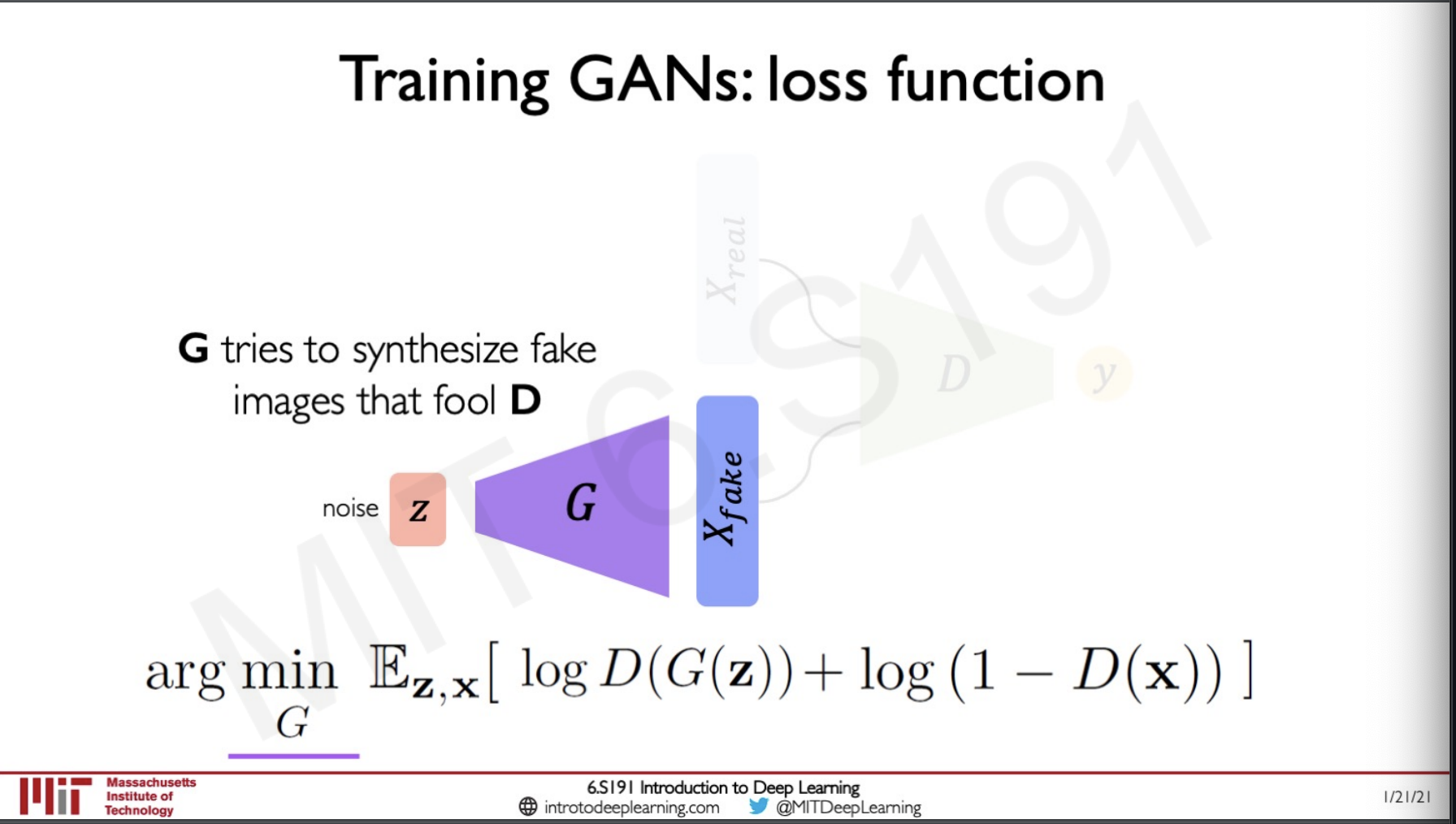
So the loss function here is to minimise the same loss term for the disciminator.

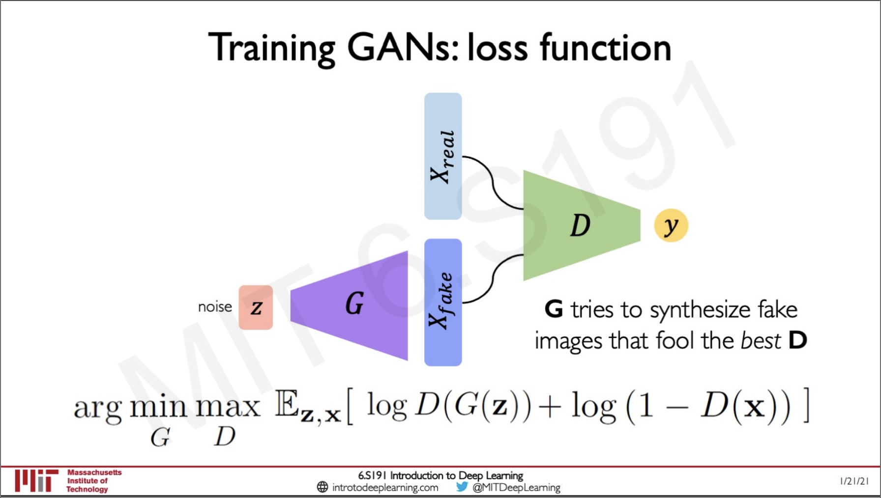
Here we can see that the network as a whole is put together in a min max kind of fashion to train the whole network.

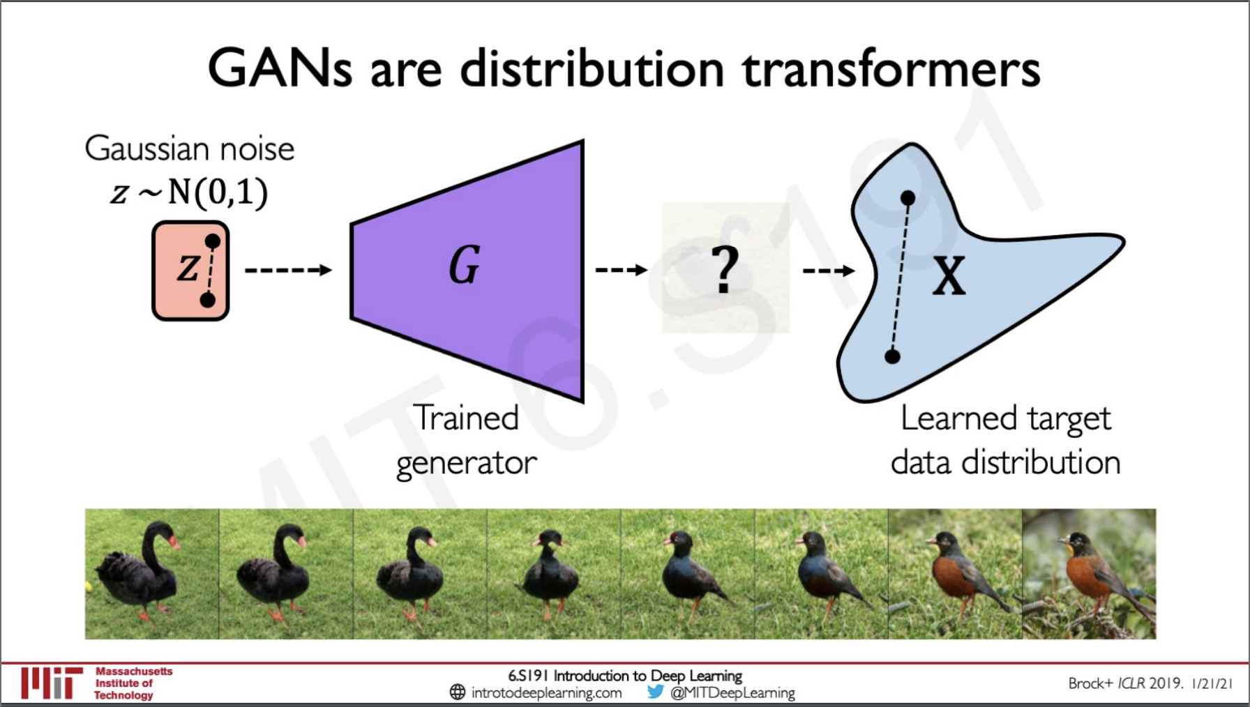
After the network is fully trained we can just take out the generator and use this to synthesise new data from the learned target data distribution.

We can take any point from the gaussian noise and pass it to the generator to form a synthetic image from the distribution.

We can actually traverse through the gaussian noise to see the interpolation of the images generated by the network.

GANs Recent Advances

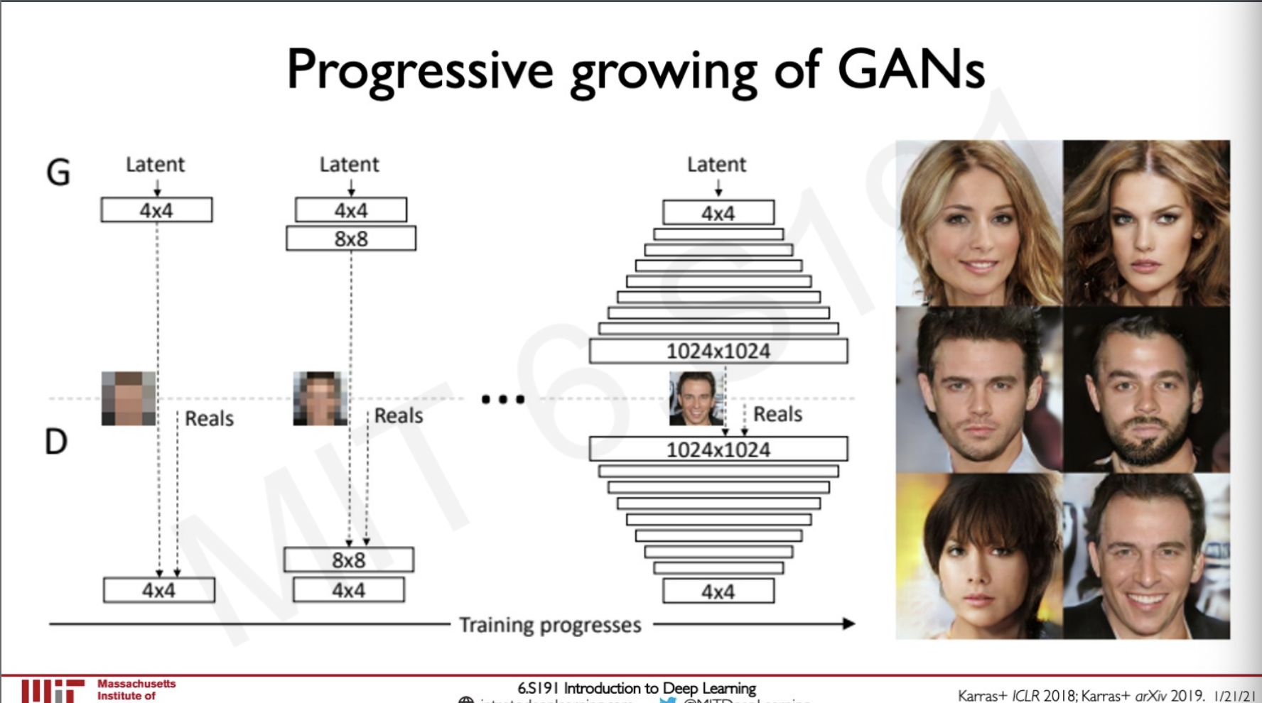
Progressive growing of GANs

These are GANs that have layers that are added to them progressively during training so that they generate better resolution images after some time steps, these GANs result in very good quality images.

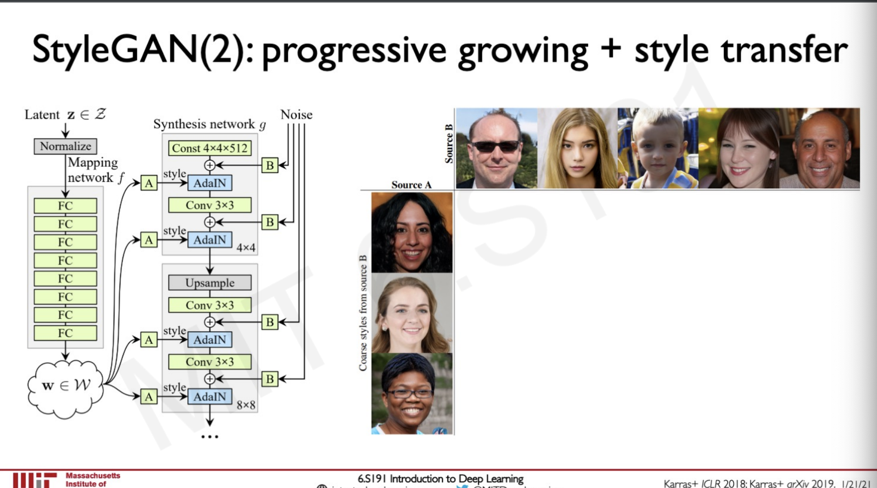
StyleGAN

This is a cross-over for the implementation of style transfer and GANs where we can generate new images by transferring the style from Images.

We can do this by taking two sources of images and using the GAN to generate a new Image with features of the two images.

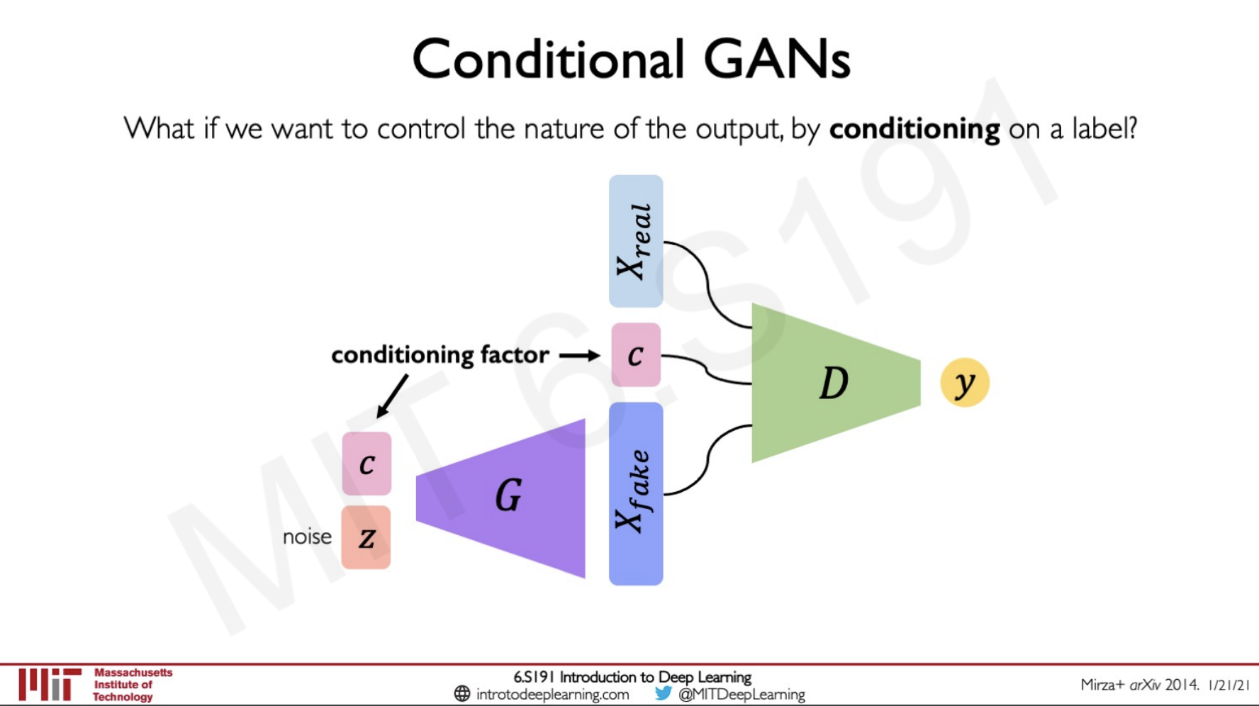
Conditional GANs

As we have seen until now the images generated by the GANs are random but this can be changed by using a conditional GAN we can choose which class of output do we need the network to generate an image for a class of our choice by introducing a condition term.

Conditional GANs and pix2pix : Paired translation

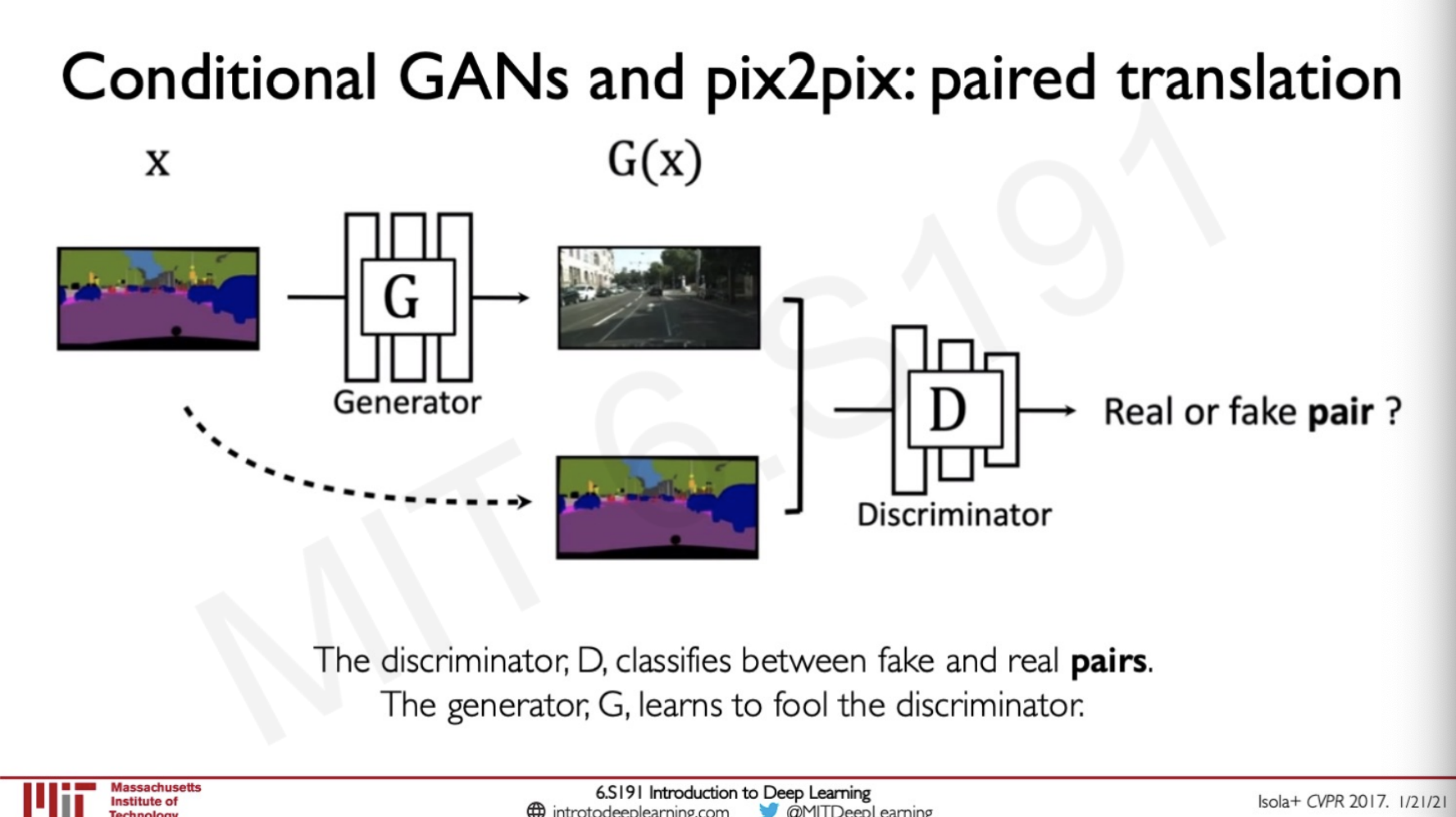
These translations can be applied in lot of fields such as Map to arial view or vice versa we can also use this for colouring from edges.

CycleGAN

Apart from paired translation we can also do unpaired data translation across domains.

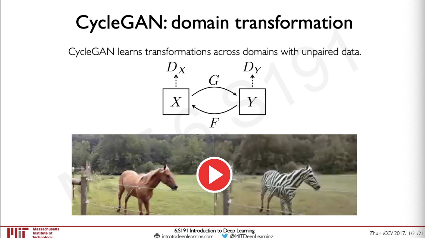
In these cases, there are two discriminators and two generators here the house skin colour to another colour. It has also done some changes in the background to make the video look more realistic.

Distribution transformations

In general GANS we transform a Gaussian noise to a target data manifold in a cycle GAN we can transform one data manifold X to another data manifold Y.

---

Sources

MIT intro deep learning : http://introtodeeplearning.com/

Slides on intro to deep learning by MIT : http://introtodeeplearning.com/slides/6S191_MIT_DeepLearning_L4.pdf

---

Lab Solutions

https://github.com/abhijitramesh/learning-introtodeeplearning/blob/main/lab2/Part2_Debiasing.ipynb

---